Introduction to graph ML : predict nodes inside graph network¶

In this exercice you are working at Twitch as a data scientist 🧙

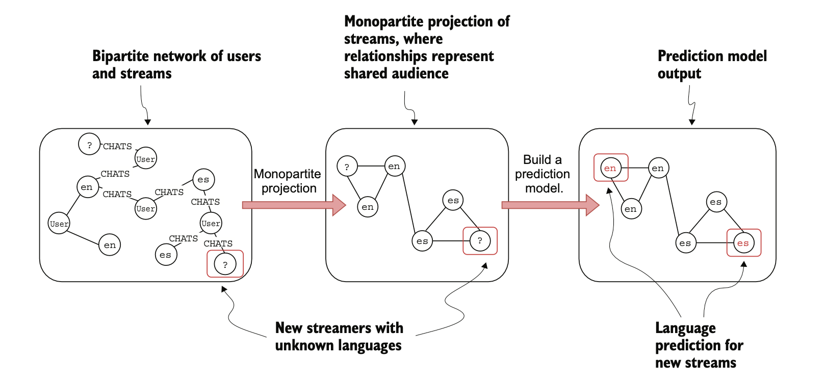
Every day, new users join the platform who decide they want to start streaming. Your manager wants you to identify the language of the new streams. Since the plat- form is worldwide, streamers likely use around 30 to 50 languages.

Let’s assume con- verting audio to text and running language-detection algorithms is not feasible for whatever reason (no so cheap)

What other way could you predict the languages of new streamers?

You can have information about users who chat in particular streams. One could hypothesize that users mostly chat in a single language. Therefore, if a user chats in two streams, it is likely that both streams are in the same language. For example, if a user is chatting in a Japanese stream and then switches a stream and interacts with the new streamer through chat, the new stream is likely in Japanese.

⚠️ There might be some exceptions with the English language, as for the most part, many people on the internet have at least a basic understanding of English. Remember, this is only an assumption that still needs to be validated ! ⚠️

First step¶

The first step in the process is to project a monopartite graph where the nodes represent streams, and the relationships represent their shared audience. The schema of the projected monopartite graph can be represented with the following Cypher statement like : (:Stream)-[:SHARED_AUDIENCE]-(:Stream).

The monopartite graph is undirected, so if stream A shares the audience with stream B, it is automatically implied that stream B also shares the audience with stream A 😇.

In addition, you can add the count of shared audiences between streamers as a relationship weight. Suppose that extracting raw data and transforming it into a monopartite graph can be done by a data engineer on your team.

In [1]:

!pip install neo4j

!pip install neo4j

Requirement already satisfied: neo4j in /Users/benj/.pyenv/versions/3.10.15/lib/python3.10/site-packages (5.28.2)
Requirement already satisfied: pytz in /Users/benj/.pyenv/versions/3.10.15/lib/python3.10/site-packages (from neo4j) (2022.7.1)

[notice] A new release of pip is available: 23.0.1 -> 25.2
[notice] To update, run: pip install --upgrade pip

First you need to connect to your neo4j docker server with your python client

check the official doc for this

In [ ]:

from neo4j import GraphDatabase

url = ""
username = ""
password = ""

# Connect to Neo4j
driver = GraphDatabase.driver(url, auth=(username, password))

from neo4j import GraphDatabase url = "" username = "" password = "" # Connect to Neo4j driver = GraphDatabase.driver(url, auth=(username, password))

In [ ]:

# print the driver object 
driver

# print the driver object driver

Out[ ]:

<neo4j._sync.driver.BoltDriver at 0x1776071c0>

Let's define a simple encapsulation function to run a cypher query into our neo4j container

In [14]:

def run_query(query):
    with driver.session() as session:
        result = session.run(query)
        return result.to_df()

def run_query(query): with driver.session() as session: result = session.run(query) return result.to_df()

Display all your databases loaded inside your docker server

In [ ]:

run_query("""
"""
)

run_query(""" """ )

Out[ ]:

	name	type	aliases	access	address	role	writer	requestedStatus	currentStatus	statusMessage	default	home	constituents
0	neo4j	standard	[]	read-write	localhost:7687	primary	True	offline	unknown		False	False	[]
1	shop	standard	[]	read-write	localhost:7687	primary	True	online	online		True	True	[]
2	system	system	[]	read-write	localhost:7687	primary	True	online	online		False	False	[]

Create a constraint named Stream

In [ ]:

run_query("""
"""
)

run_query(""" """ )

Out[ ]:

Load this twittch streamer csv https://bit.ly/3JjgKgZ and set the require properties

In [ ]:

run_query("""

"""
)

run_query(""" """ )

Out[ ]:

Load the relationship csv dataset from https://bit.ly/3S9Uyd8 representing the audience of twittch streamers and use the IN TRANSACTIONS keywork to load chunck of data instead all of it directrly

think about the relations and nodes fields you want to have for this problem

In [ ]:

# Load the data 
# 
run_query("""
""")

# Load the data # run_query(""" """)

Out[ ]:

Create a grpah projection with the neo4j gds pluging

do you think you need directed or undirected projection ? explain why ?

In [ ]:

run_query("""
"""
)

run_query(""" """ )

Out[ ]:

	nodeProjection	relationshipProjection	graphName	nodeCount	relationshipCount	projectMillis
0	{'Stream': {'label': 'Stream', 'properties': {}}}	{'SHARED_AUDIENCE': {'aggregation': 'DEFAULT',...	twitch	3721	262854	1068

Run the node2vec algo from the gds plugin on your data

check the documentation about node2vect

In [ ]:

# run query to create node2vec embeddings
run_query("""
"""
)

# run query to create node2vec embeddings run_query(""" """ )

Received notification from DBMS server: {severity: WARNING} {code: Neo.ClientNotification.Statement.FeatureDeprecationWarning} {category: DEPRECATION} {title: This feature is deprecated and will be removed in future versions.} {description: The query used a deprecated procedure. ('gds.beta.node2vec.write' has been replaced by 'gds.node2vec.write')} {position: line: 2, column: 1, offset: 1} for query: "\nCALL gds.beta.node2vec.write('twitch', \n  {embeddingDimension:8, relationshipWeightProperty:'weight',\n   inOutFactor:0.5, returnFactor:1, writeProperty:'node2vec'})\n"

Out[ ]:

	nodeCount	nodePropertiesWritten	preProcessingMillis	computeMillis	writeMillis	configuration	lossPerIteration
0	3721	3721	0	4028	347	{'writeProperty': 'node2vec', 'walkLength': 80...	[22243295.451573297]

Plot the distribution of distance of embeddings between pairs of node where relationship is present. Compare eclidiean and cosine metrics, what can you observe/conclude about these two metrics ?

Use seaborn.displot() function for a clean plot

In [ ]:

import matplotlib.pyplot as plt

plt.rcParams["figure.figsize"] = [16, 9]
import seaborn as sns

df = run_query(
)

import matplotlib.pyplot as plt plt.rcParams["figure.figsize"] = [16, 9] import seaborn as sns df = run_query( )

Out[ ]:

<seaborn.axisgrid.FacetGrid at 0x177607700>

Check the degree distribution with cosine similarity and plot it with seaborn.barplot() function

In [ ]:

df = run_query("""

"""
)

sns.barplot(data=df, x="cosineSimilarity", y="avgDegree", color="blue")

df = run_query(""" """ ) sns.barplot(data=df, x="cosineSimilarity", y="avgDegree", color="blue")

Out[ ]:

<Axes: xlabel='cosineSimilarity', ylabel='avgDegree'>

Plot the cosine similarity by the average weight degree in the network

what do you think about it ?

In [ ]:

df = run_query("""
"""
)

df = run_query(""" """ )

Out[ ]:

<Axes: xlabel='cosineSimilarity', ylabel='avgWeight'>

Export the data to a pandas dataframe in order to run a randomForest classifyer on it. You should have the result below in a tabe format 😎

You can use the pandas.factorize() function for a simple encoding

In [ ]:

import pandas as pd
data = run_query("""

"""
)

import pandas as pd data = run_query(""" """ )

In [26]:

data.head()

data.head()

Out[26]:

	streamId	language	embedding	output
0	129004176	en	[-1.7558645009994507, -1.1228911876678467, -0....	0
1	26490481	en	[-1.3582063913345337, 0.10043535381555557, -0....	0
2	213749122	en	[-1.992989182472229, -0.24940702319145203, 0.2...	0
3	30104304	en	[-1.4587347507476807, 0.6200457811355591, 0.01...	0
4	160504245	en	[-1.4484832286834717, 0.344316691160202, 0.127...	0

Instanciate a RandomForestClassifier from sklearn

In [ ]:

from sklearn.model_selection import train_test_split
from sklearn.ensemble import RandomForestClassifier

from sklearn.model_selection import train_test_split from sklearn.ensemble import RandomForestClassifier

Out[ ]:

RandomForestClassifier()

In a Jupyter environment, please rerun this cell to show the HTML representation or trust the notebook.
On GitHub, the HTML representation is unable to render, please try loading this page with nbviewer.org.

Split your dataset, train the classifier and display the classification_report

In [ ]:

from sklearn.metrics import classification_report

from sklearn.metrics import classification_report

              precision    recall  f1-score   support

           0       0.91      0.93      0.92       384
           1       0.96      0.93      0.94        54
           2       0.96      0.92      0.94        59
           3       0.84      0.82      0.83        39
           4       0.87      0.90      0.89        52
           5       0.91      0.86      0.88        58
           6       1.00      0.95      0.97        20
           7       0.93      1.00      0.96        25
           8       0.94      0.91      0.93        35
           9       0.95      0.95      0.95        19

    accuracy                           0.92       745
   macro avg       0.93      0.92      0.92       745
weighted avg       0.92      0.92      0.92       745

Display the heatmap representation of the confusion matrix

In [ ]:

from sklearn.metrics import ConfusionMatrixDisplay

from sklearn.metrics import ConfusionMatrixDisplay

Out[ ]:

<sklearn.metrics._plot.confusion_matrix.ConfusionMatrixDisplay at 0x17d120160>

Some questions to think about 🤔¶

1. What do you think about this matrix?
2. What is the appropriate metrics to select among the classification report to show your manager and why ?
3. How can you improve the classifiers quality ?