Natural Language Processing Introduction

According to Wikipedia : Natural language processing or NLP is an interdisciplinary subfield of linguistics, computer science, and artificial intelligence concerned with the interactions between computers and human language, in particular how to program computers to process and analyze large amounts of natural language data. The goal is a computer capable of "understanding" the contents of documents, including the contextual nuances of the language within them. The technology can then accurately extract information and insights contained in the documents as well as categorize and organize the documents themselves.

70 years of NLP

• 1950s : The Georgetown experiment in 1954 involved fully automatic translation of more than sixty Russian sentences into English.
• 1960s : Some notably successful NLP systems were SHRDLU, a natural language system working in restricted "blocks worlds" with restricted vocabularies, and ELIZA, a simulation of a Rogerian psychotherapist (mostly used for conjugal issues 😂) written by Joseph Weizenbaum between 1964 and 1966
• 1970s : The beginning of 'conceptual ontologies', which structured real-world information into computer-understandable data. Examples are MARGIE (Schank, 1975), SAM (Cullingford, 1978), PAM (Wilensky, 1978) and others.
• 1980s : The hey-day of symbolic methods in NLP. Focus areas of the time included research on rule-based parsing and semantics (e.g. Wilks, 1975), discourse grammars (e.g. Hobbs, 1979), and early machine translation systems such as SYSTRAN (developed by Peter Toma at Georgetown University). The 1980s also saw much work on non-symbolic approaches to NLP, including neural networks and computational linguistics as we know today. The machine-learning paradigm calls instead for using statistical inference to automatically learn such rules.
• 1990s : A resurgent interest in machine learning field with intense activity, with researchers investigating a diverse range of current topics including: corpus-based and statistical methods; computational linguistics (including parts-of-speech tagging, stemming, and parsing); information retrieval and extraction; automatic summarization, machine translation; speech recognition and generation; question answering; dialog systems; word-sense disambiguation; and information extraction, among others.
• 2000s : Due to the popularity of machine learning in the 1990s, and the popularity of kernel methods in machine learning in the 2000s, learning approaches have gained some popularity in computational linguistics. The first system using statistical machine translation was the Babylonian speech recognition system, developed by IBM in the early 1990s. The first commercial speech recognition system to be made available as a consumer product was Dragon Dictate (now known as Dragon NaturallySpeaking). The age of the first computer system to defeat a world chess champion was Deep Blue. The first computer system to defeat a Jeopardy! champion was Watson. The first computer system to defeat a world Go champion was AlphaGo. The first computer system to defeat a world StarCraft champion was AlphaStar. The first computer system to defeat a world Dota 2 champion was OpenAI Five and many others.
• 2010s : Representation learning and deep neural network-style machine learning methods became widespread in natural language processing. That popularity was due partly to a flurry of results showing that such techniques can achieve state-of-the-art results in many natural language tasks. Today is possible to pretraining large-scale language models on vast amounts of text data and then fine-tuning them on specific tasks for "cheap" (not for +100M$ like GPT 🤭). This approach allowed models to learn general language representations and demonstrated state-of-the-art performance across a wide range of NLP tasks.

Why NLP is so hard

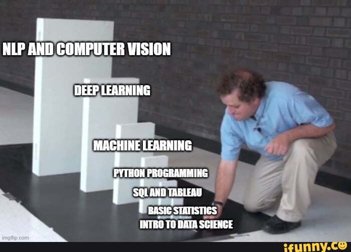
Natural language processing is considered an AI-complete problem for many reasons, first it requires solving multiple sub-problems in order to arrive at an acceptable solution for natural language understanding. Additionally, NLP research has frequent problems/challenges with :

• Text ambiguity : Language is inherently ambiguous. Words and phrases can have multiple meanings depending on the context/langage.
• Syntax and Grammar: Human languages have complex grammatical rules, exceptions and many variations.
• Contextual Understanding: The same word can have different meanings based on the surrounding words or the broader context.
• Semantic Understanding: Beyond syntax, understanding the actual meaning and semantics of words and phrases is another level of complexity. Humans have a rich understanding of word semantics, including subtle nuances and cultural references, teaching machines to grasp these nuances is challenging.

Natural Language Processing applies two techniques to help computers understand text: syntactic analysis and semantic analysis.

Syntactic analysis

Syntax refers to the arrangement of words in a sentence such that they make grammatical sense. In NLP, syntactic analysis is used to assess how the natural language aligns with the grammatical rules. Computer algorithms are used to apply grammatical rules to a group of words and derive meaning from them.

Here are some syntax techniques that can be used:

• Lemmatization: It entails reducing the various inflected forms of a word into a single form for easy analysis.
• Morphological segmentation: It involves dividing words into individual units called morphemes.
• Word segmentation: It involves dividing a large piece of continuous text into distinct units.
• Part-of-speech tagging: It involves identifying the part of speech for every word.
• Parsing: It involves undertaking grammatical analysis for the provided sentence.
• Sentence breaking: It involves placing sentence boundaries on a large piece of text.
• Stemming: It involves cutting the inflected words to their root form.
• Stop-word removal: Removes frequently occuring words that don’t add any semantic value, such as I, they, have, like, yours, etc.

Semantic analysis

Semantic analysis focuses on capturing the meaning of text. First, it starts by reading all of the words in content to capture the real meaning of any text. It identifies the text elements and assigns them to their logical and grammatical role. It analyzes context in the surrounding text and it analyzes the text structure to accurately disambiguate the proper meaning of words that have more than one definition.

Here are some techniques in semantic analysis:

• Named entity recognition (NER): It involves determining the parts of a text that can be identified and categorized into preset groups. Examples of such groups include names of people and names of places.
• Word sense disambiguation: It involves giving meaning to a word based on the context.
• Natural language generation: It involves using databases to drive semantic intentions and convert them into human language.
• Relationship extraction: Attempts to understand how entities (places, persons, organizations, etc) relate to each other in a text.

Tokenization, pre-processing and encoding

Machine Learning algorithms and computers in general don’t process text directly. So, in order to make our input data comprehensible the first task we have is to convert them to numerical vectors.

First, we have to tokenize our data. Tokenization is a common task in NLP that consists in separating a piece of text into smaller units called tokens. Tokens can be either words, characters, or subwords. Humans learn a language by connecting sound to the meaning. Machines can’t do that, so they need to be given the most basic units of text to process it better.

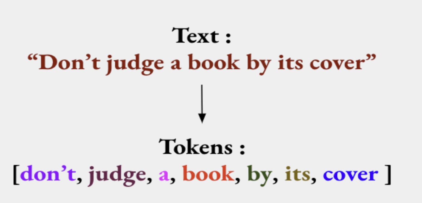
The following tokens are then used to prepare a vocabulary. The vocabulary can be constructed by considering each unique token in the corpus or by considering the top K Frequently Occurring Words and the rest are set to Unknown. Once the vocabulary is set, we proceed to encoding our text sequence into indices. The tensors of indices are padded with to the longest sequence in the batch unless we precise the sequence lenght, so all sequences have the same size.

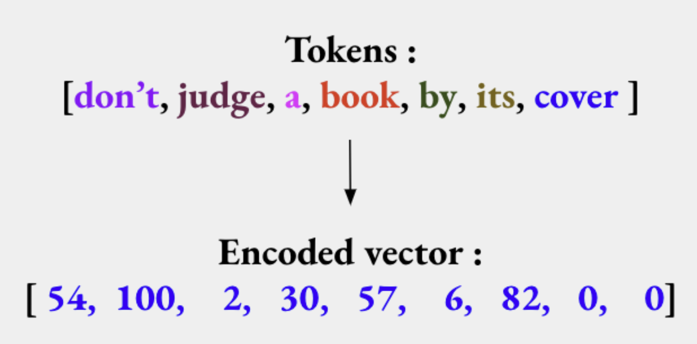
This is done to make the computation more efficient and we now have a ton of techniques to do that (in our previous example we have used a white space tokenization as you have seen).

To tokenize text in Python, we can use the nltk library (Natural Language Toolkit). If you don't have nltk installed, you can install it using the following command:

pip install nltk

Once nltk is installed on your machine, you can use it to tokenize some text like this:

import nltk
nltk.download('punkt')  # Download required data

from nltk.tokenize import word_tokenize, sent_tokenize

text = "This is a sample sentence. Tokenization is an important NLP task."
sentences = sent_tokenize(text)
words = word_tokenize(text)

print(sentences)
print(words)

You should have this output :

['This is a sample sentence.', 'Tokenization is an important NLP task.']
['This', 'is', 'a', 'sample', 'sentence', '.', 'Tokenization', 'is', 'an', 'important', 'NLP', 'task', '.']

Text preprocessing

Text preprocessing involves cleaning and transforming text data to improve its quality and make it suitable for analysis. Some common preprocessing steps include converting text to lowercase, removing punctuation, and removing stop words (common words like "the," "is," etc.). Here's an example of basic text preprocessing with the same example :

import string
from nltk.corpus import stopwords
nltk.download('stopwords')  # Download required data

def preprocess_text(text):
    # Convert text to lowercase
    text = text.lower()

    # Remove punctuation
    text = text.translate(str.maketrans('', '', string.punctuation))

    # Remove stopwords
    stop_words = set(stopwords.words('english'))
    tokens = word_tokenize(text)
    filtered_tokens = [word for word in tokens if word not in stop_words]

    return filtered_tokens

text = "This is a sample sentence. Tokenization is an important NLP task."
preprocessed_text = preprocess_text(text)
print(preprocessed_text)

and then the output should be :

['sample', 'sentence', 'tokenization', 'important', 'nlp', 'task']

As you can see, the text has been converted to lowercase, punctuation has been removed, and stop words have been removed.

Encoding text data

As you already know, computers do not process text data directly. So, in order to make our input data comprehensible for our machine the first task we have to do is to convert them to numerical value (we call this : vectors). Let's see some techniques to do that and simple python implementations.

One-hot encoding

One-hot encoding is a simple technique that encodes each word in a document as a vector with a length equal to the number of words in the vocabulary. The vector contains all zeros except for the element at the index of the word in the vocabulary. Here's an example of one-hot encoding in Python:

from sklearn.preprocessing import OneHotEncoder
from nltk.tokenize import word_tokenize

# Sample sentence
sentence = "I love natural language processing."

# Tokenize the sentence
tokens = word_tokenize(sentence)

# Create the vocabulary (unique words)
vocabulary = list(set(tokens))

# Create the OneHotEncoder object
encoder = OneHotEncoder(sparse=False)

# Reshape the tokens to a column vector
tokens_reshaped = [[token] for token in tokens]

# Perform one-hot encoding
one_hot_matrix = encoder.fit_transform(tokens_reshaped)

# Print the one-hot encoding for each word
for word_index, word in enumerate(tokens):
    word_encoding = one_hot_matrix[word_index]
    print(f"{word}: {word_encoding}")

You should see this output :

I: [0. 1. 0. 0. 0. 0. 0.]
love: [0. 0. 0. 0. 0. 1. 0.]
natural: [1. 0. 0. 0. 0. 0. 0.]
language: [0. 0. 1. 0. 0. 0. 0.]
processing: [0. 0. 0. 1. 0. 0. 0.]    

One-Hot Encoding has limitations when applied to large vocabularies as it results in high-dimensional and sparse vectors. Hence, it is less efficient for larger text corpora.

Word Frequencies

Word Frequencies encoding assigns a weight to each word based on its frequency in the document or corpus. The idea is to capture the importance of words based on their occurrence. This is a simple implementation of word frequencies encoding in Python:

from collections import Counter
from nltk.tokenize import word_tokenize

# Sample document
document = "This is a sample document. It contains repeated words."

# Tokenize the document
tokens = word_tokenize(document)

# Calculate the word frequencies
word_frequencies = Counter(tokens)

# Print the word frequencies
for word, frequency in word_frequencies.items():
    print(f"{word}: {frequency}")

You should see this output:

This: 1
is: 1
a: 1
sample: 1
document: 2
.: 1
It: 1
contains: 1
repeated: 1
words: 1

Word Frequencies encoding provides a simple representation of the importance of words based on their frequency. However, it does not consider the contextual or semantic meaning of the words.

These traditional encoding methods, such as One-Hot Encoding and Word Frequencies, were popular before the rise of statistical models. While they may have limitations compared to more advanced techniques, they offer a foundational understanding of encoding principles in NLP.

TF-IDF

TF-IDF is short for term frequency–inverse document frequency. It’s designed to reflect how important a word is to a document in a collection or corpus. The TF-IDF value increases proportionally to the number of times a word appears in the document and is offset by the number of documents in the corpus that contain the word, which helps to adjust for the fact that some words appear more frequently in general. It is one of the most popular term-weighting schemes in information retrieval because it has been shown to work well in many applications and it is relatively simple to code and compute.

Term Frequency (TF): The term Frequency (TF) measures the frequency of a term in a document. It represents how often a term occurs within a specific document. Mathematically, the TF of a term is calculated as:

\[TF(t,d)=\sum_{k}\frac{n_{k\,d}}{n_{k\,d}}\]

Where \(n_{k,d}\) is the number of times the term \(t\) occurs in the document \(d\) and \(n_{k,d}\) is the total number of terms in the document \(d\).

Inverse Document Frequency (IDF): Inverse Document Frequency (IDF) measures the importance of a term in the entire corpus. It quantifies how much information a term provides. Mathematically, the IDF of a term is calculated as:

\[IDF(t)=\log\left({\frac{N}{d f(t)}}\right)\]

Where \(N\) is the total number of documents in the corpus and \(d f(t)\) is the number of documents in the corpus that contain the term \(t\).

TF-IDF is computed by multiplying the TF and IDF values together. \(\(T F-I D F(t, d)=T F(t, d) \times I D F(t)\)\)

Enough theory, let's dive into a simple example of TF-IDF in Python 😎

from sklearn.feature_extraction.text import TfidfVectorizer

# Sample documents
documents = [
    "This is the first document.",
    "This document is the second document.",
    "And this is the third one.",
    "Is this the first document?",
]

# Create the TfidfVectorizer object
vectorizer = TfidfVectorizer()

# Perform TF-IDF encoding
tfidf_matrix = vectorizer.fit_transform(documents)

# Get the feature names (terms)
feature_names = vectorizer.get_feature_names()

# Print the TF-IDF value for each term in each document
for doc_index, doc in enumerate(documents):
    print(f"Document #{doc_index + 1}:")
    for term_index, term in enumerate(feature_names):
        tfidf_value = tfidf_matrix[doc_index, term_index]
        if tfidf_value > 0:
            print(f"{term}: {tfidf_value}")
    print()

You should see this output:

Document #1:
document: 0.6633689723434505
first: 0.46979138539904683
is: 0.37447645613334725
the: 0.37447645613334725
this: 0.37447645613334725

Document #2:
document: 0.9335416463256479
is: 0.24948598282166212
second: 0.37380847040149366
the: 0.18723822806667362
this: 0.18723822806667362

Document #3:
and: 0.49922158978027904
is: 0.3351757452359195
one: 0.49922158978027904
the: 0.3351757452359195
third: 0.49922158978027904
this: 0.49922158978027904

Document #4:
document: 0.6633689723434505
first: 0.46979138539904683
is: 0.37447645613334725
the: 0.37447645613334725
this: 0.37447645613334725

There are a ton of ways to apply TF-IDF : document retrieval, text classification, clustering, etc. It's a very powerful technique that people have useed a lot. But it can also be limited in some cases. For example, it doesn't take into account the order of the words in the document or the semantic meaning of the words 🤔

Bag of words

The Bag-of-Words (BoW) encoding is a simple and widely used technique in NLP. It represents text data as a collection of words, disregarding the order and structure of the sentences. Here's how you can implement a simple BoW encoding with the scikit-learn library :

from sklearn.feature_extraction.text import CountVectorizer

# Sample documents
documents = [
    "This is the first document.",
    "This document is the second document.",
    "And this is the third one.",
    "Is this the first document?",
]

# Create the CountVectorizer object
vectorizer = CountVectorizer()

# Perform BoW encoding
bow_matrix = vectorizer.fit_transform(documents)

# Get the feature names (words)
feature_names = vectorizer.get_feature_names()

# Print the BoW encoding for each document
for doc_index, doc in enumerate(documents):
    print(f"Document #{doc_index + 1}:")
    for term_index, term in enumerate(feature_names):
        bow_value = bow_matrix[doc_index, term_index]
        if bow_value > 0:
            print(f"{term}: {bow_value}")
    print()

As you have seen we use a CountVectorizer object from the sklearn.feature_extraction.text module, specifically designed for text feature extraction. It is used to convert a collection of text documents into a matrix of token counts. Then, the fit_transform() method of the CountVectorizer object is called with the documents list as the input. This method performs the BoW encoding on the input documents and returns a matrix representation of the token counts. Each row in the bow_matrix corresponds to a document, and each column represents a unique term (word) from the documents.

You should see this output :

Document #1:
document: 1
first: 1
is: 1
the: 1
this: 1

Document #2:
document: 2
is: 1
second: 1
the: 1
this: 1

Document #3:
and: 1
is: 1
one: 1
the: 1
third: 1
this: 1

Document #4:
document: 1
first: 1
is: 1
the: 1
this: 1

Text representations

As you know, the most basic step for the majority of NLP tasks is to convert words into numbers for machines to understand & decode patterns in a language. We call this step text representation. This step, though iterative, plays a significant role in deciding features for your machine learning model/algorithm. Let's take a look at differents text representations techniques.

In this section, we will focus on discrete text representation, where words are represented by their corresponding indexes to their position in a dictionary from a larger corpus or corpora.

Tree representations

Tree representations, such as parse trees or syntax trees, are used to analyze the grammatical structure of sentences. The nltk library in Python provides functionality to generate and visualize parse trees. Here's an example:

import nltk
from nltk import pos_tag
from nltk import RegexpParser
from nltk.tokenize import word_tokenize
nltk.download('averaged_perceptron_tagger')  # Download required data

# Sample sentence
sentence = "John loves Mary."

# Tokenize the sentence and perform part-of-speech tagging
tokens = word_tokenize(sentence)
pos_tags = pos_tag(tokens)

# Define a grammar for noun phrases
grammar = "NP: {<DT>?<JJ>*<NN>}"

# Create a parser based on the defined grammar
parser = RegexpParser(grammar)

# Generate the parse tree
tree = parser.parse(pos_tags)

# Display the parse tree
tree.pretty_print()

and you should see this output :

             S                 
    _________|_______________   
John/NNP loves/VBZ Mary/NNP ./.

Word embeddings

Word embeddings are vector representations of words that capture semantic and contextual informations. They map words to numerical vectors (encoding) where each value in the vector represents a specific feature or attribute of the word. Word embeddings are typically learned from large amounts of text data using unsupervised learning algorithms. They are used in various NLP tasks such as text classification, information retrieval, and machine translation. We will cover the two types of word embeddings in more detail below.

Pre-trained word embeddings

Pre-trained word embeddings are word embeddings that have been trained on large corpora and made available for general use. These embeddings capture general word meanings and relationships and can be readily used in various NLP tasks.

Sometimes training embeddings from scratch is not feasible due to data or computational limitations. In these cases, you can use pre-trained embeddings. Gensim provides many pre-trained models that can be loaded easily. Let's take a look at a simple example using pre-trained GloVe embeddings in python with the gensim library.

from gensim.models import KeyedVectors
import gensim.downloader as api

# Load pre-trained word-vectors from gensim-data
glove_model = api.load("glove-wiki-gigaword-100") # or word2vec-google-news-300, fasttext-wiki-news-subwords-300, etc.

# Get word embeddings for specific words
word_embedding = glove_model['cat']

# Perform operations with word embeddings
similarity = glove_model.similarity('cat', 'dog')
most_similar = glove_model.most_similar('king')

print(f"Word embedding for 'cat': {word_embedding}")
print(f"Similarity between 'cat' and 'dog': {similarity}")
print(f"Most similar words to 'king': {most_similar}")

You should see this output :

Word embedding for 'cat': [ 0.23088    0.28283    0.6318    -0.59411   -0.58599    0.63255
  0.24402   -0.14108    0.060815  -0.7898    -0.29102    0.14287
  0.72274    0.20428    0.1407     0.98757    0.52533    0.097456
  0.8822     0.51221    0.40204    0.21169   -0.013109  -0.71616
  0.55387    1.1452    -0.88044   -0.50216   -0.22814    0.023885
  0.1072     0.083739   0.55015    0.58479    0.75816    0.45706
 -0.28001    0.25225    0.68965   -0.60972    0.19578    0.044209
 -0.31136   -0.68826   -0.22721    0.46185   -0.77162    0.10208
  0.55636    0.067417  -0.57207    0.23735    0.4717     0.82765
 -0.29263   -1.3422    -0.099277   0.28139    0.41604    0.10583
  0.62203    0.89496   -0.23446    0.51349    0.99379    1.1846
 -0.16364    0.20653    0.73854    0.24059   -0.96473    0.13481
 -0.0072484  0.33016   -0.12365    0.27191   -0.40951    0.021909
 -0.6069     0.40755    0.19566   -0.41802    0.18636   -0.032652
 -0.78571   -0.13847    0.044007  -0.084423   0.04911    0.24104
  0.45273   -0.18682    0.46182    0.089068  -0.18185   -0.01523
 -0.7368    -0.14532    0.15104   -0.71493  ]
Similarity between 'cat' and 'dog': 0.8798074722290039
Most similar words to 'king': [('prince', 0.7682329416275024), ('queen', 0.7507690787315369), ('son', 0.7020888328552246), ('brother', 0.6985775828361511), ('monarch', 0.6977890729904175), ('throne', 0.691999077796936), ('kingdom', 0.6811409592628479), ('father', 0.6802029013633728), ('emperor', 0.6712858080863953), ('ii', 0.6676074266433716)]

Custom word embeddings

Training word embeddings from scratch allows you to learn word representations specific to your task or domain. One popular algorithm for training word embeddings is Word2Vec. The Word2Vec algorithm is one of the most popular techniques to learn word embeddings using a shallow neural network. It was developed by Tomas Mikolov in 2013 at Google. It comes in two flavors, the Continuous Bag of Words (CBOW) and the Skip-Gram model.

• CBOW Model: This model predicts the current word given the context. It takes the context ("the cat over the") as input and tries to predict the target word "jumps". It's faster and has slightly better accuracy for frequent words.
• Skip-Gram model: This model predicts the surrounding context words for a given word. It does the opposite of CBOW. Takes the target word "jumps" as input and tries to predict the context ("the cat over the"). It works well with small amount of data and is found to represent rare words well.

Let's take a look at a simple example using Word2Vec in python.

#train word2vec 
from gensim.models import Word2Vec
from nltk.tokenize import word_tokenize

# Sample sentences
sentences = [
    "I love natural language processing and cats.",
    "Word embeddings are so cool",
    "I love dogs also",
    "Machine learning is dope.",
]

# Tokenize the sentences
tokenized_sentences = [word_tokenize(sent.lower()) for sent in sentences]

# Train the Word2Vec model
model = Word2Vec(tokenized_sentences,vector_size=150, window=5, min_count=1, workers=4)

# Get the word embedding vector for a word
word = "love"
embedding = model.wv[word]

#most_similar = model.wv.most_similar('love')
similarity = model.wv.similarity('cats', 'dogs')

print(f"Word: {word}")
print(f"Embedding size: {embedding.shape[0]}")
print(f"Embedding values: {embedding}")
print(f"Similarity between 'cat' and 'dog': {similarity}")

You should see this output :

Embedding size: 150
Embedding values: [-4.7939620e-03  2.8219270e-03  1.4422623e-03  4.9604764e-03 ...]
Similarity between 'cat' and 'dog': 0.09130397439002991

You can change the vector_size parameter to modify the size of the embedding vector matching your specific use case. The window parameter defines the maximum distance between the current and predicted word within a sentence. The min_count parameter specifies the minimum number of occurrences of a word within the corpus. The workers parameter defines the number of threads to use while training the model.

You can notice the similarity between 'cat' and 'dog' is very low. This is because the model was trained on a very small corpus rather than a large corpus of text like we did with GloVe 🤓.

Document embeddings (aka Paragraph Vector)

Doc2Vec, also known as Paragraph Vectors, was introduced by Le and Mikolov in 2014 just one year after Word2Vec. Like his predecessor, Doc2Vec is an unsupervised algorithm that generates vectors for sentence/paragraphs/documents. This algorithm represents each document by a dense numeric vector which is learned by predicting the context in the document. We can view Doc2Vec as an extension of Word2Vec.

The objective of Doc2Vec is to create vector representations of documents that capture the meanings of the words in the documents and preserve their order it can be very useful for certain specific tasks like document classification, sentiment analysis, etc. To do this, Doc2Vec extends the Word2Vec methodology of creating word embeddings and applies it to entire documents.

There are two main approaches in the Paragraph Vector method:

• Distributed Memory (PV-DM): This is pretty much the model analogous to Continuous-bag-of-words Word2Vec. The paragraph vectors are obtained by training a neural network on the task of predicting a probability distribution of words in a paragraph given a randomly-sampled word from the paragraph.
• Distributed Bag of Words (PV-DBOW): This is the analogous of Skip-gram Word2Vec. The paragraph vectors are obtained by training a neural network on the task of predicting a probability distribution of words in a paragraph given a randomly-sampled word from the paragraph.

In the Doc2Vec model, every paragraph is mapped to a unique vector, represented by a column in matrix \(D\) and every word is also mapped to a unique vector, represented by a column in matrix \(W\). The paragraph vector and word vectors are averaged or concatenated to predict the next word in a context. The context is a sliding window that moves across the paragraph we can view this process like a convolution filter in a CNN.

To be more concrete, let's denote the paragraph vector by \(v_{(D, i)}\), and the word vectors in context by \(v_{(W, j)}\). In the PV-DM model, the prediction task for the next word given a context can be mathematically written as:

\[y = softmax((v_{(D, i)} + \sum_j v_{(W, j)}) \cdot W')\]

where W' is the weight matrix connecting the hidden layer to the output layer of the neural network, and softmax is the softmax activation function.

In the PV-DBOW model, the prediction task for the next word given a context can be mathematically written as:

\[y = softmax(v_{(D, i)} \cdot W')\]

where \(W'\) is the weight matrix connecting the hidden layer to the output layer of the neural network, and softmax is the classical softmax activation function. Both models are trained using stochastic gradient descent and backpropagation as you should expect.

Enoug theory, let's code 😂 Let's take a look at a simple example using Doc2Vec in python, you can see it is not that different from Word2Vec. Let's use the gensim's Doc2Vec to pretrain a model on a dummy corpus : our list below and generate document embeddings for it.

from gensim.models.doc2vec import Doc2Vec, TaggedDocument
from nltk.tokenize import word_tokenize

# Sample data
data = [
    "I love machine learning. Its awesome.",
    "I love coding in Python.",
    "I love building chatbots.",
    "Chatbots are very helpful in automating tasks.",
    "Python is a versatile language.",
    "Python is widely used in data science.",
    "Data science is an exciting field.",
    "Machine learning is a part of data science.",
]

# Preprocessing and tokenizing data
tagged_data = [TaggedDocument(words=word_tokenize(_d.lower()), tags=[str(i)]) for i, _d in enumerate(data)]

# Training the model with vector size=20, min_count=1 (words with frequency less than 1 are ignored)
# epochs=100 (number of iterations over the corpus)
model = Doc2Vec(tagged_data, vector_size=20, min_count=1, epochs=100)

# Print the vector of document at index 0 in data
print(model.docvecs['0'])

We first tokenize and tag the documents using TaggedDocument. Each document is tagged with a unique identifier (in this case, we just use the index of the document in the list). Then, we create a Doc2Vec model and train it on the tagged documents. The trained model can be used to retrieve the document vectors using the tags.

Like wordS, you can compute document similarity which can be useful for precise document classification tasks.

Visualizing Word Embeddings

Visualizing word embeddings can help us understand their structure and relationships. Indeed a vector representation is not easy to interpret with a human eye. One common approach is to reduce the dimensionality of the word embeddings and visualize them in a 2D or 3D space. We have two common techniques to do this:

• Principal Component Analysis (PCA): PCA is a statistical method that is used to reduce the number of dimensions in the dataset. It does this by identifying the principal components that capture the maximum variance in the data.
• t-Distributed Stochastic Neighbor Embedding (t-SNE): t-SNE is a technique for dimensionality reduction that is particularly well-suited for the visualization of high-dimensional datasets. Unlike PCA, it is a non-linear dimensionality reduction technique, which makes it more suitable for capturing the complex structure of high-dimensional data.

First we need to install some helpers lib :

pip install matplotlib sklearn gensim wget

Then we can run the following code to download the pre-trained GloVe embeddings and visualize them.

import numpy as np
import matplotlib.pyplot as plt
from sklearn.manifold import TSNE
from gensim.models import KeyedVectors
import gensim.downloader as api

# Load pre-trained word-vectors from gensim-data
glove_vectors = api.load("glove-wiki-gigaword-100") # or word2vec-google-news-300, fasttext-wiki-news-subwords-300, etc.

# Select a subset of words for visualization
words = ['cat', 'dog', 'king', 'queen', 'happy', 'sad']

# Get word embeddings for selected words
word_embeddings = [glove_vectors[word] for word in words]

# Reduce dimensionality using t-SNE
tsne = TSNE(n_components=2, random_state=42)
embeddings_2d = tsne.fit_transform(word_embeddings)

# Plot the word embeddings
plt.figure(figsize=(10, 8))
for i, word in enumerate(words):
    x, y = embeddings_2d[i]
    plt.scatter(x, y, marker='o', color='b')
    plt.text(x, y, word, fontsize=12)
plt.xlabel('Dimension 1')
plt.ylabel('Dimension 2')
plt.title('Word Embeddings Visualization')
plt.show()

You should see this output graph :

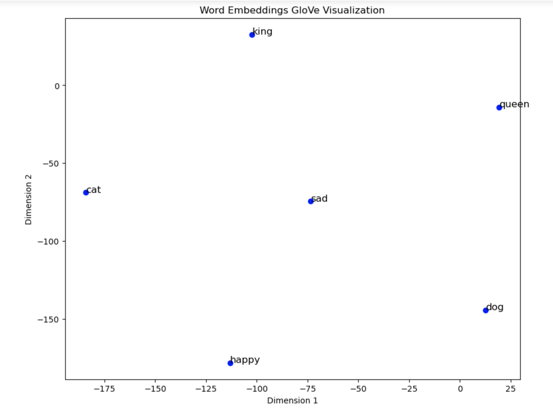
This is not very clear, but we can see that the words 'king' and 'queen' are close to each other, as well as 'cat' and 'dog'. This is because the embeddings were trained on a large corpus of text, and the model was able to learn a particular relationships between these words.

Understanding word embeddings similarity

Word similarity is one of the most common applications of word embeddings. To understand how word similarity is computed, we need to understand the concept of vector space and cosine similarity.

Let's start with the concept of vector space first 🤓. In the "word embeddings worl", each unique word is represented as a vector in n-dimensional space as we have seen earlier. Then words that share common contexts in the corpus (like our cats and dog in our previous example) are positioned in close proximity to one another in the space (or not if your training is not enought). So semantically similar words are mapped to comparatively nearby points like we have seen in the previous graph.

Now let's talk about measure of the semantic similarity between two word vectors. The common measured is the Cosine Similarity. The cosine similarity between two vectors \(A\) and \(B\) is a measure that calculates the cosine of the angle between them like in high school. Note thaht this metric is a measurement of orientation and not magnitude like in physics.

Cosine Similarity formula :

\[ \mathrm{similarity(A,B)}=\mathrm{cos}(\theta)={\frac{\bf A\cdot B}{||\mathbf{A}|||\mathbf{B}||}}={\frac{\sum_{i=1}^{n}A_{i}B_{i}}{\sqrt{\sum_{i=1}^{n}A_{i}^{2}}\sqrt{\sum_{i=1}^{n}B_{i}}}}, \]

Where:

• \(A.B\) is the dot product of A and B,
• \(||A||\) is the norm (or length) of the vector A,
• \(||B||\) is the norm (or length) of the vector B.

The cosine similarity will range from -1 to 1, with -1 meaning that the vectors are diametrically opposed, 0 meaning the vectors are orthogonal (or not related), and 1 meaning that the vectors are identical.

The importance of measurement

The choice of a distance measure (also known as a similarity measure) can significantly influence the results of your NLP tasks that rely on comparing word or document vectors.

Depending on how you've represented your text data, different measures might be more appropriate. For example, if you've represented your documents as sets of words (bag-of-words model), the Jaccard index might be a good measure of similarity. But if you've represented your documents as continuous vectors (TF-IDF or word embeddings), then cosine similarity or Euclidean distance might be more appropriate 🤔

In high-dimensional spaces, Euclidean distance can suffer from the "curse of dimensionality," where distances become less meaningful because they tend to converge. This is often the case with sparse vectors like one-hot encodings or bag-of-words models.

Some measures might be more interpretable than others, depending on the application. For example, Jaccard similarity is very interpretable for set representations: it's just the number of items in common divided by the total number of unique items. Cosine similarity can be interpreted as the cosine of the angle between two vectors, which can be a meaningful metric for text data. Certain measures are more computationally efficient than others. For large-scale applications, this might be an important factor to consider 🎯

Euclidean distance

Also known as L2 distance, it is one of the most basic metrics to calculate distance. It measures the 'as-the-crow-flies' distance. The formula to calculate Euclidean distance between two points \(v_1\) and \(v_2\) in a \(N\) dimensional vector space is:

\[d_{Euclidean}=\sqrt{\textstyle{\sum_{i=1}^{d}(v1_{i}-v2_{i})^{2}}}\]

Euclidean distance is a good measure when the embeddings are on a similar scale.

Manhattan distance

Also known as L1 distance, it is another basic metric to calculate distance. It measures the distance between two points along the axes. The formula to calculate Manhattan distance between two points \(x\) and \(y\) in a \(N\) dimensional vector space is:

\[ d_{Manhattan} = \sum_{i=1}^{N}|x_{i}-y_{i}| \]

You can think of it as the distance between two points in a city if you are not allowed to take a diagonal path and can only walk along orthogonal directions like the picture below.

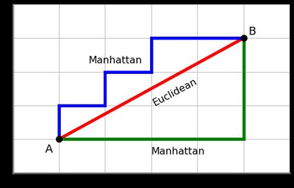
This measure could be used when difference in each dimension matters more than the actual distance between the points 🤓

Minkowski Distance

Minkowski distance is a generalization of both Euclidean and Manhattan distances. It allows for different values of the parameter \(p\), which control the level of norm used. When \(p=2\), it represents the Euclidean distance, and when \(p=1\), it represents the Manhattan distance. By varying p, we can adjust the emphasis on different dimensions and measure distance accordingly.

The Minkowski distance between two word vectors, \(v1\) and \(v2\), of dimensionality \(d\), with parameter \(p\), is given by:

\[{\mathrm{Minkowski_Distance}}=\left(\sum_{i=1}^{d}|v{\bf1}_{i}-v2_{i}|^{p}\right)^{\frac{1}{p}}\]

Cosine Distance

While cosine similarity is commonly used to measure the similarity between word vectors, cosine distance can also be used as a measure of dissimilarity. Cosine distance is simply the complement of cosine similarity. It calculates the angle between two vectors and is inversely proportional to their similarity.

The cosine distance between two word vectors, v1 and v2, can be calculated using the following formula: $$ Cosine Distance = 1 − Cosine Similarity $$

Jaccard Similarity and Hamming Distance

Jaccard Similarity or Intersection over Union is a statistic used for comparing the similarity and diversity of sample sets. It is defined as the size of the intersection divided by the size of the union of the sample sets. It's used when the embeddings are sets of items (like words in a document) rather than continuous vectors.

Hamming distance between two strings of equal length is the number of positions at which the corresponding symbols are different. It's used when the embeddings are binary vectors (like one-hot encodings) rather than continuous vectors.

These alternative distance measures provide different perspectives on the similarity or dissimilarity between word embeddings. It's important to know that the choice of a good distance metric largely depends on the problem domain you are trying to solve and of course the characteristics of your data. Do not be effraid to experiment and choose the distance metric that suits your NLP task 🤓

Let's tackle the different distance metrics and use scipy to compute them (because we are lazy and we do not want to reinvent the wheel 😅)

from scipy.spatial import distance

# Let's say we have two vectors v1 and v2
v1 = np.array([1, 2, 3])
v2 = np.array([4, 5, 6])

# Euclidean distance
euclidean_distance = distance.euclidean(v1, v2)

# Manhattan distance
manhattan_distance = distance.cityblock(v1, v2)

# Cosine distance
cosine_distance = distance.cosine(v1, v2)

# Jaccard distance - for this we'll need binary vectors, let's say bv1 and bv2
bv1 = np.array([1, 1, 0])
bv2 = np.array([1, 0, 0])
jaccard_distance = distance.jaccard(bv1, bv2)

# Hamming distance - also needs binary vectors
hamming_distance = distance.hamming(bv1, bv2)

and now let's plot the results in a simple bar chart in order to see the differences between the different distance metrics

import numpy as np
import matplotlib.pyplot as plt
from scipy.spatial import distance

def plot_distances(v1, v2):
    distance_measures = ['Euclidean', 'Manhattan', 'Cosine', 'Jaccard', 'Hamming']
    distances = [distance.euclidean(v1, v2),
                 distance.cityblock(v1, v2),
                 distance.cosine(v1, v2),
                 distance.jaccard(v1 > 0, v2 > 0),
                 distance.hamming(v1 > 0, v2 > 0)]

    # Plotting
    plt.figure(figsize=(10, 6))
    plt.bar(distance_measures, distances)
    plt.xlabel('Distance Measure')
    plt.ylabel('Distance')
    plt.title('Comparison of Distance Measures')
    plt.show()

# Example usage
v1 = np.array([1, 2, 3])
v2 = np.array([4, 5, 6])
plot_distances(v1, v2)

You should get something like this:

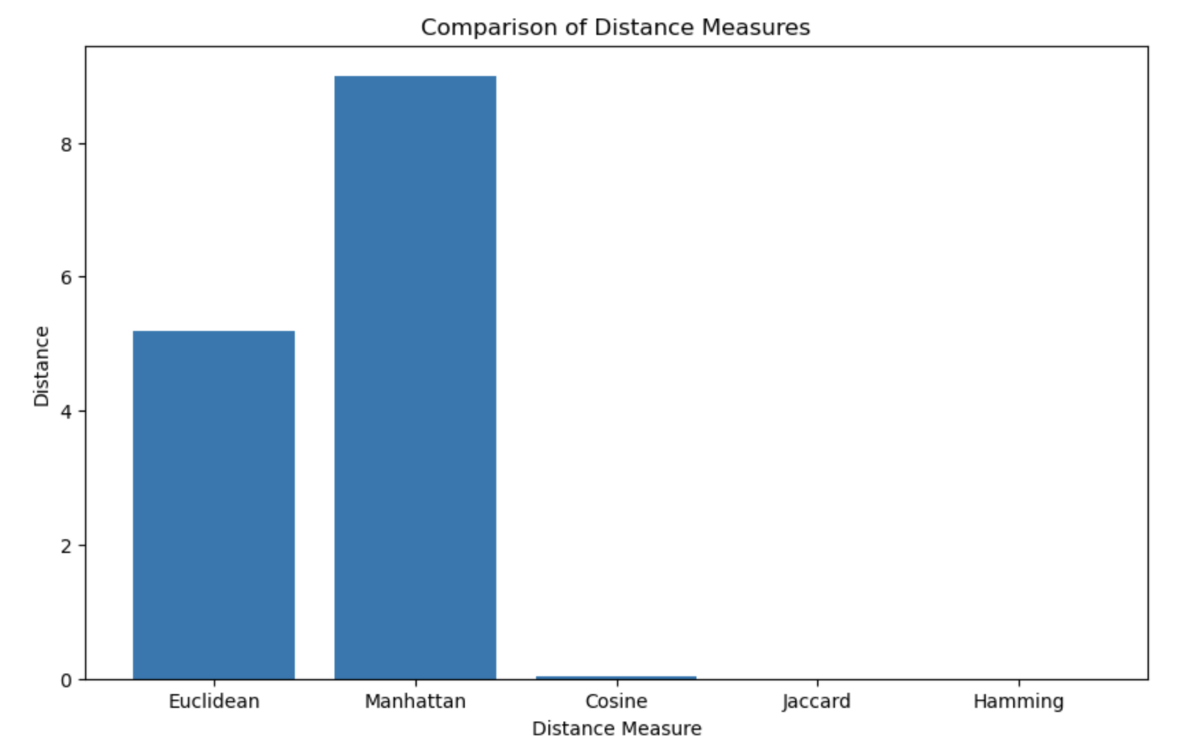
The hamming and jaccard distances are not very meaningful for continuous vectors as you can see on the graph but they are very useful for binary vectors and sets of items.

Congrats! You now know how to compute vectors from text and how to measure the distance between them. You are now ready to tackle the next section where we will learn how to use these vectors to solve NLP tasks 🥳