SVM
Support Vector Machines (SVM) are a set of supervised learning methods used for classification, regression, and outliers detection. They are particularly well-suited for classification of complex but small- or medium-sized datasets.
The fundamental idea behind SVM is to find a hyperplane that best divides a dataset into classes. The objective is to select a hyperplane with the maximum possible margin between support vectors in the given dataset. SVM searches for the maximum marginal hyperplane in the following way:
- The data is plotted in an n-dimensional space (where n is the number of features).
- Then, we perform classification by finding the hyperplane that best divides the dataset into classes.
Linear SVM some technical details
For a linearly separable dataset, the goal is to find the optimal hyperplane that separates the classes. The equation of a hyperplane is given by : $$w^Tx - b = 0$$
where $w$ is the normal vector to the hyperplane. The distance between the hyperplane and the nearest data point from either set is known as the margin. The objective is to maximize the margin. The points that lie on the margin are known as support vectors. The margin can be computed as : $$\frac{2}{\|w\|}$$
The optimization problem can be stated as : $$\min_{w,b} \frac{1}{2} \|w\|^2$$ $$\text{subject to } y_i(w^Tx_i - b) \geq 1, \forall i$$
where $y_i$ is the class label of the $i^{th}$ example. The above optimization problem can be solved using Lagrange multipliers. The solution to the above problem can be written as : $$w = \sum_{i=1}^N \alpha_i y_i x_i$$
where $\alpha_i$ are the Lagrange multipliers. The decision function for a new example $x$ can be written as : $$f(x) = \sum_{i=1}^N \alpha_i y_i x_i^Tx - b$$
Non-linear SVM
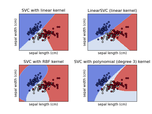
In many real-world scenarios, data is not linearly separable. To handle such cases, SVM uses a technique called the kernel trick. The main idea is to map the input data into a higher-dimensional space where it becomes linearly separable. A kernel function computes the dot product of the transformed vectors.
Commonly used kernel functions include :
- Linear : $\langle x, x'\rangle$.
- Polynomial : $(\gamma \langle x, x'\rangle + r)^d$. $d$ is specified by keyword degree, $r$ by coef0.
- RBF : $\exp(-\gamma \|x-x'\|^2)$. $\gamma$ is specified by keyword gamma, must be greater than 0.
- Sigmoid : $\tanh(\gamma \langle x,x'\rangle + r)$, where $r$ is specified by coef0.
The effect of the kernel can be seen in the following figure :

SVM in scikit-learn
from mpl_toolkits import mplot3d
from sklearn.datasets import make_circles
from sklearn.svm import SVC
import numpy as np
import matplotlib.pyplot as plt
from scipy import stats
from ipywidgets import interact, fixed
import seaborn as sns; sns.set()
def plot_svc_decision_function(model, ax=None, plot_support=True):
    if ax is None:
        ax = plt.gca()
    xlim = ax.get_xlim()
    ylim = ax.get_ylim()

   # create grid to evaluate model
    x = np.linspace(xlim[0], xlim[1], 30)
    y = np.linspace(ylim[0], ylim[1], 30)
    Y, X = np.meshgrid(y, x)
    xy = np.vstack([X.ravel(), Y.ravel()]).T
    P = model.decision_function(xy).reshape(X.shape)

   # plot decision boundary and margins
    ax.contour(X, Y, P, colors='k',
              levels=[-1, 0, 1], alpha=0.5,
              linestyles=['--', '-', '--'])

   # plot support vectors
    if plot_support:
        ax.scatter(model.support_vectors_[:, 0],
        model.support_vectors_[:, 1],
        s=300, linewidth=1, facecolors='none');
    ax.set_xlim(xlim)
    ax.set_ylim(ylim)
X, y = make_circles(100, factor=.1, noise=.1)
r = np.exp(-(X ** 2).sum(1))
clf = SVC(kernel='linear').fit(X, y)
plt.scatter(X[:, 0], X[:, 1], c=y, s=50, cmap='autumn')
plot_svc_decision_function(clf, plot_support=False);
def plot_3D(elev=30, azim=30, X=X, y=y):
    ax = plt.subplot(projection='3d')
    ax.scatter3D(X[:, 0], X[:, 1], r, c=y, s=50, cmap='autumn')
    ax.view_init(elev=elev, azim=azim)
    ax.set_xlabel('x')
    ax.set_ylabel('y')
    ax.set_zlabel('r')

interact(plot_3D, elev=0, azip=(-180, 180), X=fixed(X), y=fixed(y));
interactive(children=(IntSlider(value=0, description='elev', max=1), IntSlider(value=30, description='azim', m…
Advantages and Disadvantages
Advantages
- Effective in high-dimensional spaces.
- Uses a subset of training points (support vectors), making it memory efficient.
- Versatile due to the use of different kernel functions.
Disadvantages
- Not suitable for large datasets due to high training time.
- Less effective on noisier datasets with overlapping classes.
Support Vector Machines offer a powerful way to perform linear and non-linear classification. By using the kernel trick, SVMs can handle complex datasets that aren't linearly separable in their original space. However, careful consideration is needed when choosing the kernel function and parameters to ensure optimal performance.