K-Means¶

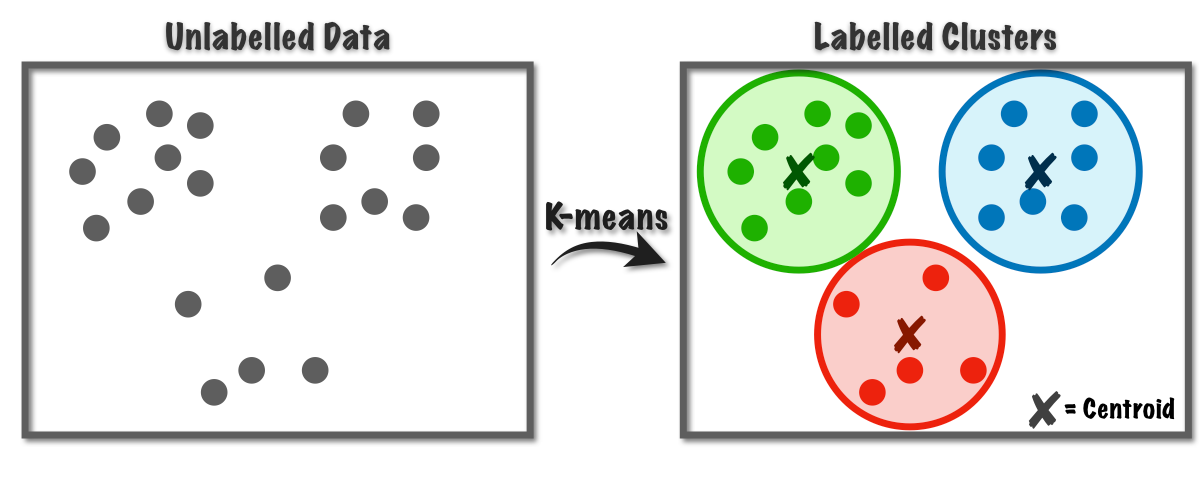
K-means is one of the simplest and most popular unsupervised machine learning algorithms. The goal of K-means is to group similar data points together and discover underlying patterns. To achieve this objective, K-means looks for a fixed number (k) of clusters in a dataset.

A cluster refers to a collection of data points aggregated together because of certain similarities. The 'K' in K-means represents the number of clusters the algorithm tries to identify in the dataset.

Algorithm idea¶

The K-means algorithm works iteratively to assign each data point to one of $k$ groups based on the features provided.

Steps:

• Initialization: Randomly initialize $k$ centroids.
• Assignment: Assign each data point to the nearest centroid. This forms the clusters.
• Update: Calculate the new means (centroids) of each cluster.
• Repeat: Repeat steps 2 and 3 until the centroids do not change significantly.

Mathematically, the objective of the K-means clustering is to minimize the within-cluster sum of squares (WCSS). It can be represented as : $$\mathrm{WCSS}=\textstyle{\sum_{i=1}^{k}}\sum_{x\in C_{i}}|x-\mu_{i}||^{2}$$ where $C_{i}$ is the $i$th cluster and $\mu_{i}$ is the centroid of the $i$th cluster and x is a data point in cluster $C_{i}$.

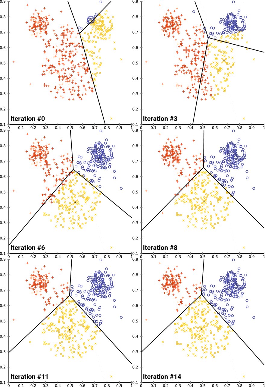
This is an animation of the K-means algorithm in action. Notice how the centroids (black cross) move with each iteration 🤓

Example in scikit-learn¶

In [1]:

import pandas as pd 
import numpy as np 
import matplotlib.pyplot as plt 
import seaborn as sns

import pandas as pd import numpy as np import matplotlib.pyplot as plt import seaborn as sns

In [2]:

from sklearn.datasets import load_iris
iris = load_iris()

from sklearn.datasets import load_iris iris = load_iris()

In [9]:

X = iris.data
y = iris.target

X = iris.data y = iris.target

In [10]:

from sklearn.cluster import KMeans
# Applying KMeans to the Mall dataset
kmeans = KMeans(n_clusters= 3, init= "k-means++", max_iter=300, n_init = 10, random_state=0)
y_kmeans = kmeans.fit_predict(X)

from sklearn.cluster import KMeans # Applying KMeans to the Mall dataset kmeans = KMeans(n_clusters= 3, init= "k-means++", max_iter=300, n_init = 10, random_state=0) y_kmeans = kmeans.fit_predict(X)

In [37]:

# Visualizing the clusters and centroids
plt.scatter(X[y == 0,2], X[y == 0,3], s = 100, c = 'red')
plt.scatter(X[y == 1,2], X[y == 1,3], s = 100, c = 'green')
plt.scatter(X[y == 2,2], X[y == 2,3], s = 100, c = 'blue')
plt.scatter(kmeans.cluster_centers_[:,2], kmeans.cluster_centers_[:,3], s = 300, c = 'yellow', label = 'centroids')
plt.title('clusters of iris')
plt.xlabel('petal width')
plt.ylabel('Sepal length')
plt.legend()
plt.show()

# Visualizing the clusters and centroids plt.scatter(X[y == 0,2], X[y == 0,3], s = 100, c = 'red') plt.scatter(X[y == 1,2], X[y == 1,3], s = 100, c = 'green') plt.scatter(X[y == 2,2], X[y == 2,3], s = 100, c = 'blue') plt.scatter(kmeans.cluster_centers_[:,2], kmeans.cluster_centers_[:,3], s = 300, c = 'yellow', label = 'centroids') plt.title('clusters of iris') plt.xlabel('petal width') plt.ylabel('Sepal length') plt.legend() plt.show()

In [40]:

# Visualisation with dimension reduction
from sklearn.decomposition import PCA
reduced_data = PCA(n_components=2).fit_transform(X)
kmeans = KMeans(init='k-means++', n_clusters=3, n_init=10)
kmeans.fit(reduced_data)

# Visualisation with dimension reduction from sklearn.decomposition import PCA reduced_data = PCA(n_components=2).fit_transform(X) kmeans = KMeans(init='k-means++', n_clusters=3, n_init=10) kmeans.fit(reduced_data)

Out[40]:

KMeans(algorithm='auto', copy_x=True, init='k-means++', max_iter=300,
    n_clusters=3, n_init=10, n_jobs=1, precompute_distances='auto',
    random_state=None, tol=0.0001, verbose=0)

In [47]:

plt.scatter(reduced_data[y == 0,0], reduced_data[y == 0,1], s = 100, c = 'red')
plt.scatter(reduced_data[y == 1,0], reduced_data[y == 1,1], s = 100, c = 'green')
plt.scatter(reduced_data[y == 2,0], reduced_data[y == 2,1], s = 100, c = 'blue')
plt.scatter(kmeans.cluster_centers_[:,0], kmeans.cluster_centers_[:,1], s = 300, c = 'yellow')

plt.scatter(reduced_data[y == 0,0], reduced_data[y == 0,1], s = 100, c = 'red') plt.scatter(reduced_data[y == 1,0], reduced_data[y == 1,1], s = 100, c = 'green') plt.scatter(reduced_data[y == 2,0], reduced_data[y == 2,1], s = 100, c = 'blue') plt.scatter(kmeans.cluster_centers_[:,0], kmeans.cluster_centers_[:,1], s = 300, c = 'yellow')

Out[47]:

<matplotlib.collections.PathCollection at 0x1a1e400748>

Choosing $k$¶

One of the challenges with K-means is that we need to specify the number of clusters (k) before running the algorithm 😅. Several methods can help determine the optimal number of clusters:

• Elbow Method: Plot the number of clusters against the WCSS. The point where the reduction in WCSS begins to slow down (elbow point) is considered a good estimate for 'k'.
• Silhouette Method: Measures the quality of clusters. A higher silhouette score indicates better-defined clusters.

Advantages and Disadvantages¶

Advantages¶

• Simple and easy to implement.
• Efficient in terms of computational cost.
• Scales well to large datasets.

Disadvantages¶

• Assumes clusters to be spherical and equally sized.
• Sensitive to the initial placement of centroids.
• Can get stuck in local optima. Often, multiple runs with different initializations are required.
• Requires the number of clusters to be specified beforehand.

Variations and Improvements¶

• K-means++: Improves the initialization of the centroids to provide better convergence.
• Mini Batch K-means: Uses a random sample of data points in each iteration for updating the clusters, making it faster.
• Bisecting K-means: A hierarchical approach where clusters are split iteratively.

In [48]:

# Using the Elbow method to find the optimal number K of clusters
from sklearn.cluster import KMeans
wcss =  []
for i in range (1,11): 
    kmeans = KMeans(n_clusters= i, init = "k-means++", max_iter = 300, n_init = 10, random_state = 0)
    kmeans.fit(X)
    wcss.append(kmeans.inertia_)
plt.plot(range(1,11), wcss)
plt.title('Elbow Method')
plt.xlabel('Number of Clusters')
plt.ylabel('WCSS')
plt.show()

# Using the Elbow method to find the optimal number K of clusters from sklearn.cluster import KMeans wcss = [] for i in range (1,11): kmeans = KMeans(n_clusters= i, init = "k-means++", max_iter = 300, n_init = 10, random_state = 0) kmeans.fit(X) wcss.append(kmeans.inertia_) plt.plot(range(1,11), wcss) plt.title('Elbow Method') plt.xlabel('Number of Clusters') plt.ylabel('WCSS') plt.show()

Metrics for evaluating clustering performance¶

There are several metrics for evaluating clustering performance. We will use the following metrics in this notebook :

• Homogeneity: A clustering result satisfies homogeneity if all of its clusters contain only data points which are members of a single class.
• Completeness: A clustering result satisfies completeness if all the data points that are members of a given class are elements of the same cluster.
• V-measure: The V-measure is the harmonic mean between homogeneity and completeness.
• Silhouette Coefficient: The Silhouette Coefficient is calculated using the mean intra-cluster distance (a) and the mean nearest-cluster distance (b) for each sample. The Silhouette Coefficient for a sample is (b - a) / max(a, b). To clarify, b is the distance between a sample and the nearest cluster that the sample is not a part of. Note that Silhouette Coefficient is only defined if number of labels is 2 <= n_labels <= n_samples - 1.

Implementation of Silhouette Coefficient in scikit-learn¶

In [51]:

from sklearn.datasets import make_blobs
from sklearn.cluster import KMeans
from sklearn.metrics import silhouette_samples, silhouette_score
import matplotlib.cm as cm


for n_clusters in range(2,4):
    # Create a subplot with 1 row and 1 columns
    fig, ax1 = plt.subplots(1, 1)
    fig.set_size_inches(18, 7)

    # The 1st subplot is the silhouette plot
    # The silhouette coefficient can range from -1, 1 but in this example all
    # lie within [-0.1, 1]
    ax1.set_xlim([-0.1, 1])
    # The (n_clusters+1)*10 is for inserting blank space between silhouette
    # plots of individual clusters, to demarcate them clearly.
    ax1.set_ylim([0, len(X) + (n_clusters + 1) * 10])

    # Initialize the clusterer with n_clusters value and a random generator
    # seed of 10 for reproducibility.
    clusterer = KMeans(n_clusters=n_clusters, random_state=10)
    cluster_labels = clusterer.fit_predict(X)

    # The silhouette_score gives the average value for all the samples.
    # This gives a perspective into the density and separation of the formed
    # clusters
    silhouette_avg = silhouette_score(X, cluster_labels)
    print("For n_clusters =", n_clusters,
          "The average silhouette_score is :", silhouette_avg)

    # Compute the silhouette scores for each sample
    sample_silhouette_values = silhouette_samples(X, cluster_labels)

    y_lower = 10
    for i in range(n_clusters):
        # Aggregate the silhouette scores for samples belonging to
        # cluster i, and sort them
        ith_cluster_silhouette_values = \
            sample_silhouette_values[cluster_labels == i]

        ith_cluster_silhouette_values.sort()

        size_cluster_i = ith_cluster_silhouette_values.shape[0]
        y_upper = y_lower + size_cluster_i

        color = cm.nipy_spectral(float(i) / n_clusters)
        ax1.fill_betweenx(np.arange(y_lower, y_upper),
                          0, ith_cluster_silhouette_values,
                          facecolor=color, edgecolor=color, alpha=0.7)

        # Label the silhouette plots with their cluster numbers at the middle
        ax1.text(-0.05, y_lower + 0.5 * size_cluster_i, str(i))

        # Compute the new y_lower for next plot
        y_lower = y_upper + 10  # 10 for the 0 samples

    ax1.set_title("The silhouette plot for the various clusters.")
    ax1.set_xlabel("The silhouette coefficient values")
    ax1.set_ylabel("Cluster label")

    # The vertical line for average silhouette score of all the values
    ax1.axvline(x=silhouette_avg, color="red", linestyle="--")

    ax1.set_yticks([])  # Clear the yaxis labels / ticks
    ax1.set_xticks([-0.1, 0, 0.2, 0.4, 0.6, 0.8, 1])

plt.show()

from sklearn.datasets import make_blobs from sklearn.cluster import KMeans from sklearn.metrics import silhouette_samples, silhouette_score import matplotlib.cm as cm for n_clusters in range(2,4): # Create a subplot with 1 row and 1 columns fig, ax1 = plt.subplots(1, 1) fig.set_size_inches(18, 7) # The 1st subplot is the silhouette plot # The silhouette coefficient can range from -1, 1 but in this example all # lie within [-0.1, 1] ax1.set_xlim([-0.1, 1]) # The (n_clusters+1)*10 is for inserting blank space between silhouette # plots of individual clusters, to demarcate them clearly. ax1.set_ylim([0, len(X) + (n_clusters + 1) * 10]) # Initialize the clusterer with n_clusters value and a random generator # seed of 10 for reproducibility. clusterer = KMeans(n_clusters=n_clusters, random_state=10) cluster_labels = clusterer.fit_predict(X) # The silhouette_score gives the average value for all the samples. # This gives a perspective into the density and separation of the formed # clusters silhouette_avg = silhouette_score(X, cluster_labels) print("For n_clusters =", n_clusters, "The average silhouette_score is :", silhouette_avg) # Compute the silhouette scores for each sample sample_silhouette_values = silhouette_samples(X, cluster_labels) y_lower = 10 for i in range(n_clusters): # Aggregate the silhouette scores for samples belonging to # cluster i, and sort them ith_cluster_silhouette_values = \ sample_silhouette_values[cluster_labels == i] ith_cluster_silhouette_values.sort() size_cluster_i = ith_cluster_silhouette_values.shape[0] y_upper = y_lower + size_cluster_i color = cm.nipy_spectral(float(i) / n_clusters) ax1.fill_betweenx(np.arange(y_lower, y_upper), 0, ith_cluster_silhouette_values, facecolor=color, edgecolor=color, alpha=0.7) # Label the silhouette plots with their cluster numbers at the middle ax1.text(-0.05, y_lower + 0.5 * size_cluster_i, str(i)) # Compute the new y_lower for next plot y_lower = y_upper + 10 # 10 for the 0 samples ax1.set_title("The silhouette plot for the various clusters.") ax1.set_xlabel("The silhouette coefficient values") ax1.set_ylabel("Cluster label") # The vertical line for average silhouette score of all the values ax1.axvline(x=silhouette_avg, color="red", linestyle="--") ax1.set_yticks([]) # Clear the yaxis labels / ticks ax1.set_xticks([-0.1, 0, 0.2, 0.4, 0.6, 0.8, 1]) plt.show()

For n_clusters = 2 The average silhouette_score is : 0.6808136202713507
For n_clusters = 3 The average silhouette_score is : 0.5525919445213676

Conclusion¶

K-means is a foundational algorithm for cluster analysis in data mining. Despite its simplicity, K-means can achieve robust clustering results on a wide range of datasets, especially when the shape and number of clusters are appropriate for the algorithm's assumptions. It's also computationally efficient and easy to implement. However, K-means has several drawbacks, such as the need to specify the number of clusters beforehand and the sensitivity to the initial placement of centroids.