Introduction to CNN with pytorch
import torch
import torch.nn as nn
import torch.optim as optim
import torchvision
import torchvision.transforms as transforms
from tqdm import tqdm
import matplotlib.pyplot as plt
import numpy as np
Loading our data
Here is an example of how to load the Fashion-MNIST dataset from TorchVision. Fashion-MNIST is a dataset of Zalando’s article images consisting of 60,000 training examples and 10,000 test examples. Each example comprises a 28×28 grayscale image and an associated label from one of 10 classes.
We load the FashionMNIST Dataset with the following parameters:
- root is the path where the train/test data is stored,
- train specifies training or test dataset,
- download=True downloads the data from the internet if it’s not available at root.
- transform and target_transform specify the feature and label transformations
Transformation pipeline
in order to be processed better by our algorithm, we define a standard transformation pipeline that will be applied to the images in the dataset. It uses the torchvision.transforms module, which provides several classes to perform transformations on images, such as resizing, cropping, normalization...
The transforms.Compose function takes a list of transformations and combines them into a single function that is applied to the data. Here, it includes two transformations:
transforms.ToTensor(): This converts the image, which is usually loaded as a PIL (Python Imaging Library) image, into a PyTorch tensor. It also scales the image's pixel intensity values, which are typically between 0 and 255, to be between 0 and 1.transforms.Normalize((0.5, 0.5, 0.5), (0.5, 0.5, 0.5)): This normalizes the image by subtracting the mean and dividing by the standard deviation. The arguments to the function are the means and standard deviations for each color channel. Here, (0.5, 0.5, 0.5) for both mean and standard deviation implies that it will bring the pixel values from a range of [0,1] to [-1,1].
This is a very common normalization strategy, which helps keep pixel values small and on a similar scale, which can help with the training of the neural network.
# Define the transformation above to apply
transform = transforms.Compose([
    transforms.ToTensor(),
    transforms.Normalize((0.5, 0.5, 0.5), (0.5, 0.5, 0.5))  # Normalize to range [-1, 1]
])

# Load the CIFAR10 training data
trainset = torchvision.datasets.CIFAR10(root='./data', train=True, download=True, transform=transform)
trainloader = torch.utils.data.DataLoader(trainset, batch_size=4, shuffle=True, num_workers=2)

# Load the CIFAR10 testing data
testset = torchvision.datasets.CIFAR10(root='./data', train=False, download=True, transform=transform)
testloader = torch.utils.data.DataLoader(testset, batch_size=4, shuffle=False, num_workers=2)

# Define the classes in the CIFAR10 dataset
classes = ('plane', 'car', 'bird', 'cat', 'deer', 'dog', 'frog', 'horse', 'ship', 'truck')
Files already downloaded and verified
Files already downloaded and verified
What is CNN 🤔
A Convolutional Neural Network (CNN), or ConvNet, is a type of neural network that is particularly good at processing grid-like data, such as images. These networks use a mathematical operation called convolution, which is essentially a dot product between two matrices. In the case of a CNN, these matrices are the input data (e.g., an image) and a set of learnable parameters known as a kernel or filter.
Convolution
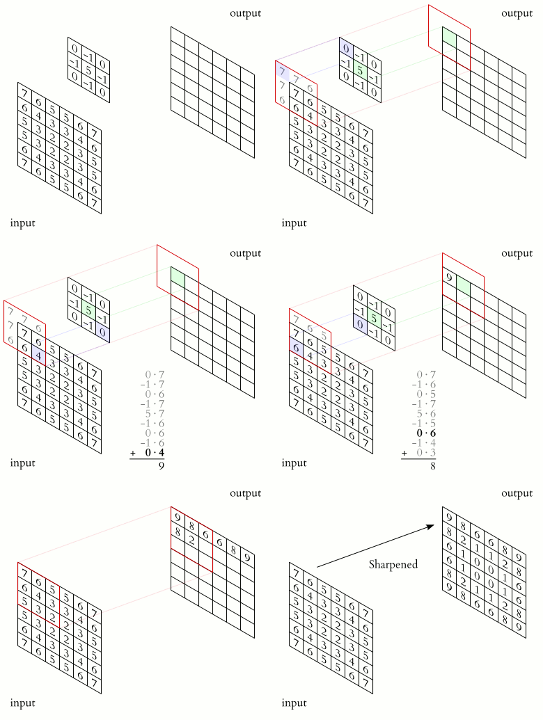
A convolution is a mathematical operation that is a special kind of linear operation. In our case we will focus on the convolution product. The idea behind it is to generalizes the idea of moving average and is the mathematical representation of the notion of linear filter. It applies both to temporal data (in signal processing for example) and to spatial data (in image processing). Because a clear image is better than a theorical explanation 🤓 :

Convolution in CNN
The convolution process in a CNN involves taking a small, square matrix of numbers (called a kernel or filter), and passing it over an input image to produce a transformed output image (called a feature map or convolved feature).
In the CNN architecture, the kernel is a set of learnable weights. During the convolution process, the kernel is moved across the image, one pixel at a time. At each position, the kernel is overlaid on a portion of the image, and a dot product operation is performed between the values in the kernel and the overlaid image pixels. The results of these dot products are summed up to produce a single pixel in the output feature map like the animation below :

CNN Architecture overview
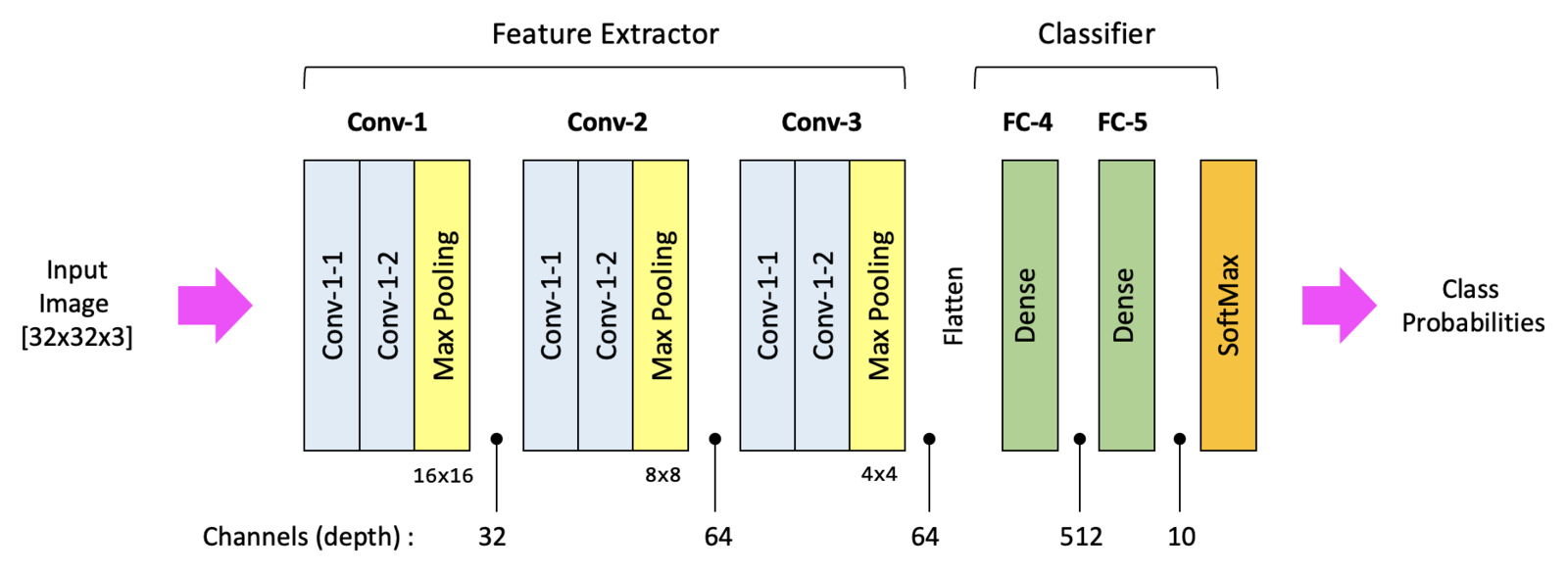
Here's a high-level overview of the major components of a CNN:
Convolution Layer
This layer performs the convolution operation, which in the context of a CNN is a dot product between the input data and a set of learnable parameters, or kernels. The kernels slide across the input data, calculating the dot product at each position, to produce an output known as an activation map. The formula for the output volume of a convolutional layer is given as:
$$W_{out} = (W - F + 2P) / S + 1$$ $$H_{out} = (H - F + 2P) / S + 1$$ $$D_{out} = K$$
Where $W$ and $H$ are the width and height of the input volume, $F$ is the size of the filter, $P$ is the padding, $S$ is the stride, and $K$ is the number of filters used.

Non-Linearity Layers (ReLU, Sigmoid, Tanh)
These layers are used to introduce non-linearity to the activation map because the convolution operation is a linear operation. The most popular non-linearity function is the Rectified Linear Unit (ReLU), which simply thresholds the input at zero (i.e., negative values are set to zero). See more details in the Deep learning section.
Pooling Layer
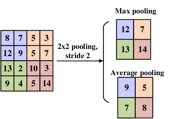
This layer reduces the spatial dimensions of the input (height and width) while maintaining the depth. It does this by applying a pooling function (like max pooling, which takes the maximum value) over the input volume. The formula for the output volume of a pooling layer is given as:
$$W_{out} = (W - F) / S + 1$$ $$H_{out} = (H - F) / S + 1$$ $$D_{out} = D$$
Where $W$ and $H$ are the width and height of the input volume, $D$ is the depth of the input volume, $F$ is the size of the filter, and $S$ is the stride. Below, here is an illustration of two famous pooling :

Fully Connected Layer (Dense)
Neurons in this layer have full connections to all activations in the previous layer. This layer is usually the last layer in a CNN and computes the class scores, which are the final output of the network.
A typical CNN architecture might look something like this:

Implementation
For our example let's simplify the architecture above by implementing only :
$$INPUT → [CONV2D + MaxPooling2D] → [CONV2D] → [FC]*3$$
Play with our data
testloader.dataset
Dataset CIFAR10
    Number of datapoints: 10000
    Root location: ./data
    Split: Test
    StandardTransform
Transform: Compose(
               ToTensor()
               Normalize(mean=(0.5, 0.5, 0.5), std=(0.5, 0.5, 0.5))
           )
type(testloader.dataset)
torchvision.datasets.cifar.CIFAR10
As you can see is not very easy to handle a torchvision.datasets object. Let's dive into it in order to print some example images of our dataset.
data_ex = iter(testloader)
data, label = next(data_ex)
- data_ex = iter(testloader): This line is creating an iterator over the DataLoader testloader. This allows us to fetch samples from it using the next function.
- data, label = next(data_ex): This line fetches the next batch from the DataLoader. The DataLoader returns a batch of images and their corresponding labels.
Now let's print the first image data :
data[0]
tensor([[[ 0.2392,  0.2471,  0.2941,  ...,  0.0745, -0.0118, -0.0902],
         [ 0.1922,  0.1843,  0.2471,  ...,  0.0667, -0.0196, -0.0667],
         [ 0.1843,  0.1843,  0.2392,  ...,  0.0902,  0.0196, -0.0588],
         ...,
         [-0.4667, -0.6706, -0.7569,  ..., -0.7020, -0.8980, -0.6863],
         [-0.5216, -0.6157, -0.7255,  ..., -0.7961, -0.7725, -0.8431],
         [-0.5765, -0.5608, -0.6471,  ..., -0.8118, -0.7333, -0.8353]],

        [[-0.1216, -0.1294, -0.0902,  ..., -0.2549, -0.2863, -0.3333],
         [-0.1216, -0.1373, -0.1059,  ..., -0.2549, -0.2863, -0.3098],
         [-0.1373, -0.1451, -0.1294,  ..., -0.2314, -0.2549, -0.3020],
         ...,
         [-0.0275, -0.2157, -0.3098,  ..., -0.2392, -0.4980, -0.3333],
         [-0.0902, -0.2000, -0.3333,  ..., -0.3569, -0.3569, -0.4980],
         [-0.1608, -0.1765, -0.3020,  ..., -0.3961, -0.3412, -0.4745]],

        [[-0.6157, -0.6314, -0.6000,  ..., -0.7176, -0.7176, -0.7412],
         [-0.6000, -0.6863, -0.6471,  ..., -0.7569, -0.7490, -0.7333],
         [-0.6314, -0.7412, -0.7176,  ..., -0.7333, -0.7333, -0.7412],
         ...,
         [ 0.3882,  0.1608,  0.0745,  ...,  0.1451, -0.1529, -0.0039],
         [ 0.3176,  0.1608,  0.0353,  ...,  0.0196, -0.0118, -0.1608],
         [ 0.2549,  0.1686,  0.0353,  ..., -0.0275,  0.0118, -0.1373]]])
data[0].shape
torch.Size([3, 32, 32])
As you may notice a torch.Tensor is not very visual 😂
So, let's transform our image in order to be able to print it with the imshow function of matplotlib :
np.transpose(data[0], (1, 2, 0))
tensor([[[ 0.2392, -0.1216, -0.6157],
         [ 0.2471, -0.1294, -0.6314],
         [ 0.2941, -0.0902, -0.6000],
         ...,
         [ 0.0745, -0.2549, -0.7176],
         [-0.0118, -0.2863, -0.7176],
         [-0.0902, -0.3333, -0.7412]],

        [[ 0.1922, -0.1216, -0.6000],
         [ 0.1843, -0.1373, -0.6863],
         [ 0.2471, -0.1059, -0.6471],
         ...,
         [ 0.0667, -0.2549, -0.7569],
         [-0.0196, -0.2863, -0.7490],
         [-0.0667, -0.3098, -0.7333]],

        [[ 0.1843, -0.1373, -0.6314],
         [ 0.1843, -0.1451, -0.7412],
         [ 0.2392, -0.1294, -0.7176],
         ...,
         [ 0.0902, -0.2314, -0.7333],
         [ 0.0196, -0.2549, -0.7333],
         [-0.0588, -0.3020, -0.7412]],

        ...,

        [[-0.4667, -0.0275,  0.3882],
         [-0.6706, -0.2157,  0.1608],
         [-0.7569, -0.3098,  0.0745],
         ...,
         [-0.7020, -0.2392,  0.1451],
         [-0.8980, -0.4980, -0.1529],
         [-0.6863, -0.3333, -0.0039]],

        [[-0.5216, -0.0902,  0.3176],
         [-0.6157, -0.2000,  0.1608],
         [-0.7255, -0.3333,  0.0353],
         ...,
         [-0.7961, -0.3569,  0.0196],
         [-0.7725, -0.3569, -0.0118],
         [-0.8431, -0.4980, -0.1608]],

        [[-0.5765, -0.1608,  0.2549],
         [-0.5608, -0.1765,  0.1686],
         [-0.6471, -0.3020,  0.0353],
         ...,
         [-0.8118, -0.3961, -0.0275],
         [-0.7333, -0.3412,  0.0118],
         [-0.8353, -0.4745, -0.1373]]])
np.transpose(data[0], (1, 2, 0)) is for reordering the dimensions of the first image in the batch.
🚧 PyTorch tensors for images usually have the shape (channels, height, width), but the imshow function from matplotlib expects the shape (height, width, channels). 🚧
The transpose operation switches the order of the dimensions to match what imshow expects.
plt.imshow(np.transpose(data[0], (1, 2, 0)))
plt.show()
Clipping input data to the valid range for imshow with RGB data ([0..1] for floats or [0..255] for integers).
It seams pretty black, let's apply a last transformation : a normalisation by dividing/2 and add 0.5 to our image.
The purpose of this normalization is to bring the pixel values of the image into the range [0, 1]. This is typically done when the image was originally normalized to have values in the range [-1, 1] (as is common with many image datasets).
test = data[0] / 2 + 0.5
plt.imshow(np.transpose(test, (1, 2, 0)))
plt.title(f'{classes[label[0]]}') #This line is setting the title of the image plot to be the class of the image (as determined by the label).
plt.show()
You can notice the poor image quality, due to data compression it do not matter for our exercice our network will be faster to train 😎
Implementing the CNN class 😎
For our implementation we will define the following architecture :
- CONV2D(in_channels:3, out_channels:6, kernel_size:5)
- MaxPooling2D(kernel_size:2, stride:2)
- CONV2D(in_channels:6, out_channels:16, kernel_size:5)
- FC(in_features: 16 * 5 * 5, out_features:120)
- FC(in_features: 120, out_features:84)
- FC(in_features: 84, out_features:10)
import torch.nn.functional as F

class BasicConvNet(nn.Module):
    """
        Define the neural network architecture.

            INPUT → [CONV2D + MaxPooling2D] → [CONV2D] → [FC]*3
    """
    def __init__(self):
        super(BasicConvNet, self).__init__()
        # Define the layers
        self.conv1 = nn.Conv2d(3, 6, 5)  # Convolutional layer
        self.pool = nn.MaxPool2d(2, 2)   # Pooling layer
        self.conv2 = nn.Conv2d(6, 16, 5) # Another convolutional layer
        self.fc1 = nn.Linear(16 * 5 * 5, 120) # Fully connected layer
        self.fc2 = nn.Linear(120, 84)    # Another fully connected layer
        self.fc3 = nn.Linear(84, 10)     # Output layer --> 10 classes

    def forward(self, x):
        """Define the forward pass operations."""

        x = self.pool(F.relu(self.conv1(x)))
        x = self.pool(F.relu(self.conv2(x)))
        x = x.view(-1, 16 * 5 * 5)
        x = F.relu(self.fc1(x))
        x = F.relu(self.fc2(x))
        x = self.fc3(x)
        return x

# Instantiate the neural network
net = BasicConvNet()
# Define the loss function and optimizer
criterion = nn.CrossEntropyLoss()
optimizer = optim.SGD(net.parameters(), lr=0.001, momentum=0.9)
# Lists to keep track of training progress
train_loss_list = []
accuracy_list = []

#sexy progress bar
from tqdm import tqdm

# loop over the dataset multiple times
for epoch in range(2):

    running_loss = 0.0
    correct = 0
    total = 0

    # We wrap the iterable object trainloader with tqdm
    pbar = tqdm(enumerate(trainloader, 0), total=len(trainloader), ncols=80, leave=False)

    for i, data in pbar:
        # get the inputs; data is a list of [inputs, labels]
        inputs, labels = data

        # zero the parameter gradients
        optimizer.zero_grad()

        # forward + backward + optimize
        outputs = net(inputs)
        loss = criterion(outputs, labels)
        loss.backward()
        optimizer.step()

        # calculate accuracy
        _, predicted = torch.max(outputs.data, 1)
        total += labels.size(0)
        correct += (predicted == labels).sum().item()

        # print statistics
        running_loss += loss.item()

        # Set the postfix of the progress bar to show loss and accuracy
        pbar.set_postfix({'Loss': running_loss / (i+1), 'Accuracy %': 100 * correct / total}, refresh=True)

        if i % 2000 == 1999:    # append loss and accuracy every 2000 mini-batches
            train_loss_list.append(running_loss / 2000)
            accuracy_list.append(100 * correct / total)
            running_loss = 0.0


# Function to evaluate model on test set
def evaluate_model(testloader, model):
    correct = 0
    total = 0
    with torch.no_grad():
        for data in testloader:
            images, labels = data
            outputs = model(images)
            _, predicted = torch.max(outputs.data, 1)
            total += labels.size(0)
            correct += (predicted == labels).sum().item()

    print('Accuracy of the network on the 10000 test images: %d %%' % (100 * correct / total))
def imshow(img):
    img = img / 2 + 0.5     # unnormalize
    npimg = img.numpy()
    plt.imshow(np.transpose(npimg, (1, 2, 0)))
    plt.show()


# Function to show a random prediction from the test set
def show_random_prediction(testloader, model, classes):
    dataiter = iter(testloader)
    images, labels = next(dataiter)
    outputs = model(images)
    _, predicted = torch.max(outputs, 1)

    imshow(torchvision.utils.make_grid(images))
    print('GroundTruth: ', ' '.join('%5s' % classes[labels[j]] for j in range(4)))
    print('Predicted: ', ' '.join('%5s' % classes[predicted[j]] for j in range(4)))

evaluate_model(testloader, net)
show_random_prediction(testloader, net, classes)

# Plotting the training progress
plt.figure(figsize=(12, 4))
plt.subplot(1, 2, 1)
plt.plot(train_loss_list, label='Loss')
plt.legend()
plt.subplot(1, 2, 2)
plt.plot(accuracy_list, label='Accuracy')
plt.legend()
plt.show()
Accuracy of the network on the 10000 test images: 53 %
GroundTruth:    cat  ship  ship plane
Predicted:    cat   car   car  ship
This is a basic example, but you can extend it with more layers, different types of layers, different training techniques, etc.
Please note 🤔
The actual architecture of a CNN (number of layers, types of layers, size of filters, etc.) depends heavily on the specific task and the dataset. You often need to experiment with different architectures to find the best one for your task.