Image processing techniques¶

Image processing involves a suite of techniques that modify and analyze digital images using computer algorithms. This pivotal step is integral to numerous applications, ranging from face recognition and object detection to image compression. The primary goal of image processing is either to enhance the quality of an image or to extract significant information from it.

This part is crucial for many Computer Vision tasks, as the right preprocessing can significantly elevate a model's performance. In this section, we will explore various image processing techniques that can be used to analyze and modify images. These techniques include image thresholding, blurring, edge detection, and computing image gradients.

Let's start by using our helper functions from the previous section and our plant stem image 😃

In [2]:

import cv2
import matplotlib.pyplot as plt
import numpy as np 

def display_image_in_notebook(img):
    # Convert the image from BGR to RGB
    img_rgb = cv2.cvtColor(img, cv2.COLOR_BGR2RGB)
    # Display the image using matplotlib
    plt.imshow(img_rgb)
    #if you want to remove the graduation on the axis
    #plt.axis('off')
    plt.show()

# Load our test image
img = cv2.imread('./data/frame_1.png', 1)

# Display the image in Jupyter notebook
display_image_in_notebook(img)

import cv2 import matplotlib.pyplot as plt import numpy as np def display_image_in_notebook(img): # Convert the image from BGR to RGB img_rgb = cv2.cvtColor(img, cv2.COLOR_BGR2RGB) # Display the image using matplotlib plt.imshow(img_rgb) #if you want to remove the graduation on the axis #plt.axis('off') plt.show() # Load our test image img = cv2.imread('./data/frame_1.png', 1) # Display the image in Jupyter notebook display_image_in_notebook(img)

Image Thresholding¶

Image thresholding is a technique for segmenting an image into different parts. It is a simple, yet effective method for separating objects from the background.

In thresholding, we select a threshold value, and then set all the pixel values less than or greater than this threshold value to a new value, effectively highlighting the portions of the image of interest.

Here is a simple Binary Thresholding on our test image

In [13]:

# Apply simple thresholding
ret, thresh1 = cv2.threshold(img, 127, 255, cv2.THRESH_BINARY)

# Display the result
display_image_in_notebook(thresh1)

# Apply simple thresholding ret, thresh1 = cv2.threshold(img, 127, 255, cv2.THRESH_BINARY) # Display the result display_image_in_notebook(thresh1)

In [4]:

#Modify and play with our simple thresholding
ret, thresh1 = cv2.threshold(img, 60, 150, cv2.THRESH_BINARY)

# Display the result
display_image_in_notebook(thresh1)

#Modify and play with our simple thresholding ret, thresh1 = cv2.threshold(img, 60, 150, cv2.THRESH_BINARY) # Display the result display_image_in_notebook(thresh1)

AdaptiveThreshold¶

Traditional thresholding applies a single threshold value to the entire image. If the pixel value is above the threshold, it's set to one value (usually white), and if it's below the threshold, it's set to another value (usually black). This method can be effective when the image has uniform illumination.

However, in many real-world scenarios, images might have varying lighting conditions across different regions. In such cases, using a global threshold might not yield the best results. This is where adaptive thresholding comes in.

Parameters¶

• src: Source image, which should be grayscale.
• maxValue: Maximum value to assign to thresholded pixels.
• adaptiveMethod: The method to determine the threshold for the current pixel
• thresholdType: The type of thresholding to be applied (usually cv2.THRESH_BINARY or cv2.THRESH_BINARY_INV).
• blockSize: Size of the neighborhood area (3x3, 5x5, 7x7, etc.). It must be an odd number.
• C: A constant subtracted from the mean or weighted mean. It's used to fine-tune the thresholding.

As mentioned, images might have different lighting conditions in different regions. Adaptive thresholding calculates the threshold for a pixel based on a small region around it. This makes it suitable for images with varying illumination. The function also allows you to choose between mean and Gaussian methods, giving you the flexibility to choose the best method for your specific image. The block size and the constant C can also be adjusted to fine-tune the results.

In [16]:

# Convert the image to grayscale
gray_img = cv2.cvtColor(img, cv2.COLOR_BGR2GRAY)

# Adaptive Thresholding
thresh2 = cv2.adaptiveThreshold(gray_img, 255, 
                                cv2.ADAPTIVE_THRESH_MEAN_C, 
                                cv2.THRESH_BINARY, 11, 2)

# Display the result
display_image_in_notebook(thresh2)

# Convert the image to grayscale gray_img = cv2.cvtColor(img, cv2.COLOR_BGR2GRAY) # Adaptive Thresholding thresh2 = cv2.adaptiveThreshold(gray_img, 255, cv2.ADAPTIVE_THRESH_MEAN_C, cv2.THRESH_BINARY, 11, 2) # Display the result display_image_in_notebook(thresh2)

Image Blurring¶

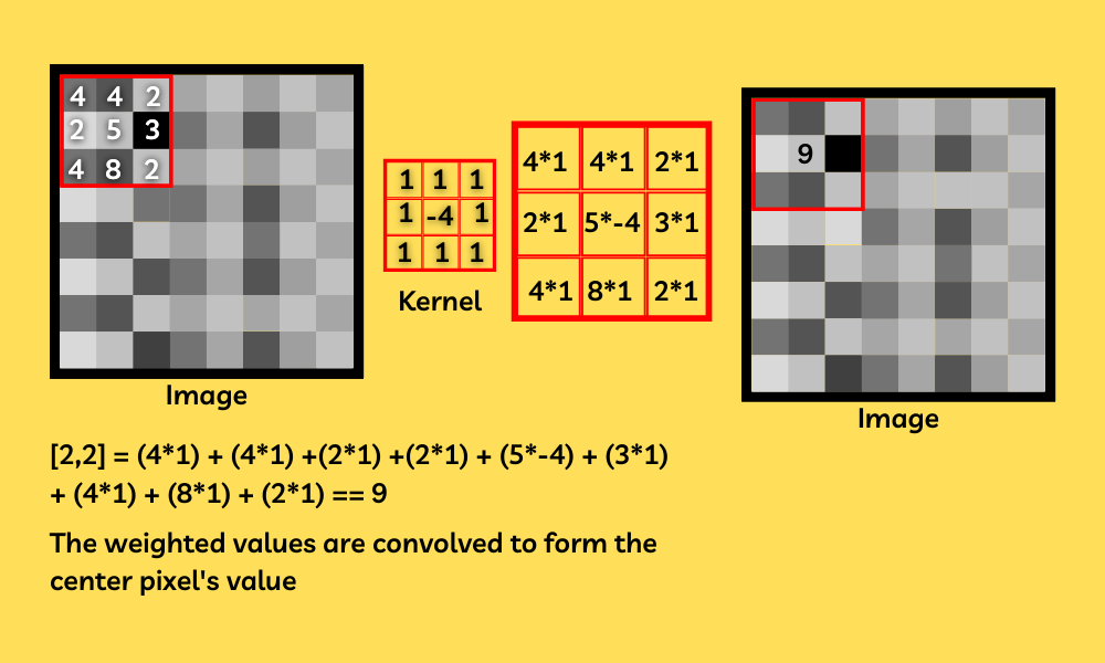
Image blurring, also known as smoothing, is the process of reducing the noise and details in an image. It's achieved by convolving the image with a filter (often called a kernel or mask as you can see in the picture above) that represents a specific type of blur.

If you want to know more about blurring I recommand you this article from geekforgeeks here

Common Blurring Techniques:¶

Average blur¶

This method involves convolving the image with a normalized box filter. It simply takes the average of all the pixels under the kernel area and replaces the central element.

Let's take a look of the effect on our image here :

In [10]:

# Load our test image
img = cv2.imread('./data/frame_1.png', 1)

# Averaging
blur = cv2.blur(img, (15,15))

# Display the result
display_image_in_notebook(img)

# Load our test image img = cv2.imread('./data/frame_1.png', 1) # Averaging blur = cv2.blur(img, (15,15)) # Display the result display_image_in_notebook(img)

Gaussian blur¶

This method uses a Gaussian kernel. It's effective in removing Gaussian noise from the image. The size of the kernel and the standard deviation (sigma) of the Gaussian determine the extent of the blur.

Let's not focus on the maths details and test it :

In [11]:

# Applying GaussianBlur
gblur = cv2.GaussianBlur(img, (15,15), 0)

# Display the result
display_image_in_notebook(gblur)

# Applying GaussianBlur gblur = cv2.GaussianBlur(img, (15,15), 0) # Display the result display_image_in_notebook(gblur)

Other techniques¶

• Median Blur : Instead of replacing the central pixel value with an average, it's replaced with the median of all the pixels under the kernel. Particularly effective against salt-and-pepper noise.
• Bilateral Filter : This method blurs the image while keeping the edges sharp. It uses two Gaussian filters: one for space (spatial weight) and another for pixel differences (intensity weight).

Image Edge Detection¶

Edge detection is a fundamental operation in image processing and computer vision. It identifies boundaries within images, helping in object recognition, feature extraction, and more. By highlighting drastic intensity changes in an image, edge detection provides a kind of abstraction that emphasizes structural properties.

Why is Edge Detection Important¶

• Feature Extraction: Edges can capture essential features in an image.
• Object Detection: Boundaries defined by edges help in distinguishing and recognizing objects.
• Reduction in Data: By focusing on edges, we can ignore less important information, making some algorithms faster and more efficient.
• Computer Vision Applications: Essential for tasks like motion detection, object tracking, and more.

Canny Edge Detection¶

The Canny Edge Detection method is one of the most popular edge detection techniques and is widely used in image processing and computer vision. It was developed by John F. Canny in 1986.

The Canny Edge Detection algorithm is a multi-stage process combining noise reduction, gradient calculation, non-maximum suppression and others. You can find more details about the algorithm here

In [16]:

# Load our test image
img = cv2.imread('./data/frame_1.png', 1)

# Applying Canny Edge detection
edges = cv2.Canny(img, 100, 200)

# Display the result
display_image_in_notebook(edges)

# Load our test image img = cv2.imread('./data/frame_1.png', 1) # Applying Canny Edge detection edges = cv2.Canny(img, 100, 200) # Display the result display_image_in_notebook(edges)

Image Gradients¶

Image gradients are a fundamental concept in image processing and computer vision. They represent the change in intensity of pixel values in an image. Gradients often point in the direction of the highest rate of change in intensity, and their magnitude can give a measure of that change.

Why Image Gradients¶

• Edge Detection: Gradients can highlight significant intensity transitions, which often correspond to edges.
• Feature Extraction: Gradients can be used to extract and describe local features in an image.
• Motion Analysis: Gradients can help in estimating motion direction in video sequences.

Several gradient operators are employed in image analysis and processing, including the Sobel, Scharr, Prewitt, and Laplacian of Gaussian (LoG) methods. Each operator possesses unique characteristics and benefits, making them apt for various tasks like identifying edges, extracting features, and segmenting images.

Sobel Operator¶

In [17]:

# Load our image in grayscale
image = cv2.imread('./data/frame_1.png', cv2.IMREAD_GRAYSCALE)

# Calculate the x and y gradients using the Sobel operator
sobel_x = cv2.Sobel(image, cv2.CV_64F, 1, 0, ksize=3)
sobel_y = cv2.Sobel(image, cv2.CV_64F, 0, 1, ksize=3)

# Convert gradient images from float64 back to uint8
sobel_x_abs = cv2.convertScaleAbs(sobel_x)
sobel_y_abs = cv2.convertScaleAbs(sobel_y)

# Combine the two gradient directions
combined = cv2.addWeighted(sobel_x_abs, 0.5, sobel_y_abs, 0.5, 0)

# Display the images
plt.subplot(2, 2, 1), plt.imshow(image, cmap='gray')
plt.title('Original Image'), plt.xticks([]), plt.yticks([])

plt.subplot(2, 2, 2), plt.imshow(sobel_x_abs, cmap='gray')
plt.title('Sobel X'), plt.xticks([]), plt.yticks([])

plt.subplot(2, 2, 3), plt.imshow(sobel_y_abs, cmap='gray')
plt.title('Sobel Y'), plt.xticks([]), plt.yticks([])

plt.subplot(2, 2, 4), plt.imshow(combined, cmap='gray')
plt.title('Combined Gradient'), plt.xticks([]), plt.yticks([])

plt.tight_layout()
plt.show()

# Load our image in grayscale image = cv2.imread('./data/frame_1.png', cv2.IMREAD_GRAYSCALE) # Calculate the x and y gradients using the Sobel operator sobel_x = cv2.Sobel(image, cv2.CV_64F, 1, 0, ksize=3) sobel_y = cv2.Sobel(image, cv2.CV_64F, 0, 1, ksize=3) # Convert gradient images from float64 back to uint8 sobel_x_abs = cv2.convertScaleAbs(sobel_x) sobel_y_abs = cv2.convertScaleAbs(sobel_y) # Combine the two gradient directions combined = cv2.addWeighted(sobel_x_abs, 0.5, sobel_y_abs, 0.5, 0) # Display the images plt.subplot(2, 2, 1), plt.imshow(image, cmap='gray') plt.title('Original Image'), plt.xticks([]), plt.yticks([]) plt.subplot(2, 2, 2), plt.imshow(sobel_x_abs, cmap='gray') plt.title('Sobel X'), plt.xticks([]), plt.yticks([]) plt.subplot(2, 2, 3), plt.imshow(sobel_y_abs, cmap='gray') plt.title('Sobel Y'), plt.xticks([]), plt.yticks([]) plt.subplot(2, 2, 4), plt.imshow(combined, cmap='gray') plt.title('Combined Gradient'), plt.xticks([]), plt.yticks([]) plt.tight_layout() plt.show()

The x-gradient (Sobel X) will highlight the vertical edges, and the y-gradient (Sobel Y) will highlight the horizontal edges in the image. The combined gradient will give a more comprehensive view of the edges in all directions.

By visualizing these gradients, now I hope you'll get a clearer understanding of how gradients capture the intensity changes and edges in an image 🤓

In [23]:

# Compute the laplacian gradient 
laplacian = cv2.Laplacian(image, cv2.CV_64F)
laplacian

# Compute the laplacian gradient laplacian = cv2.Laplacian(image, cv2.CV_64F) laplacian

Out[23]:

array([[  6.,  -5.,   6., ...,   0.,   7.,   2.],
       [  6.,  -6.,   0., ...,   3.,   4.,  -1.],
       [  1.,   4.,  -5., ...,  -2., -13.,  -3.],
       ...,
       [-18., -24., -31., ...,  -8.,  -1.,  -1.],
       [ 31.,  31.,  26., ...,  33.,   8.,   9.],
       [ 30.,  42.,  73., ..., -10., -13.,  -2.]])

Erosion and Dilation¶

Erosion and dilation are fundamental operations in the domain of morphological image processing. They are primarily used to modify the structure or shape of objects within an image. These operations are particularly useful for tasks like noise reduction, joining broken parts, and finding intensity bumps or holes in images.

Morphological Operations¶

Morphological operations process images based on their shape. They work on binary images and require two inputs: the original image and a structuring element or kernel, which decides the nature of the operation.

Erosion¶

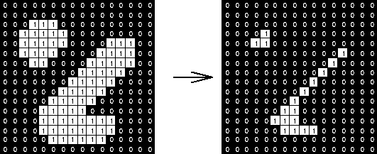
Erosion shrinks the white region (foreground) in a binary image. The basic idea is that the value of the output pixel is the minimum value of all the pixels in the input pixel's neighborhood. If any of the pixels in the kernel is 0, the pixel in the original image (under the kernel center) will be eroded (set to 0).

It's useful for removing small white noises, separating two connected objects, and eroding the boundaries of the foreground object.

In [26]:

# Erosion with kernel (5,5)
kernel = np.ones((5,5), np.uint8)
eroded_image = cv2.erode(image, kernel, iterations=1)
display_image_in_notebook(eroded_image)

# Erosion with kernel (5,5) kernel = np.ones((5,5), np.uint8) eroded_image = cv2.erode(image, kernel, iterations=1) display_image_in_notebook(eroded_image)

Dilatation¶

Dilation does the opposite of erosion: it enlarges the white region in the binary image 🤓

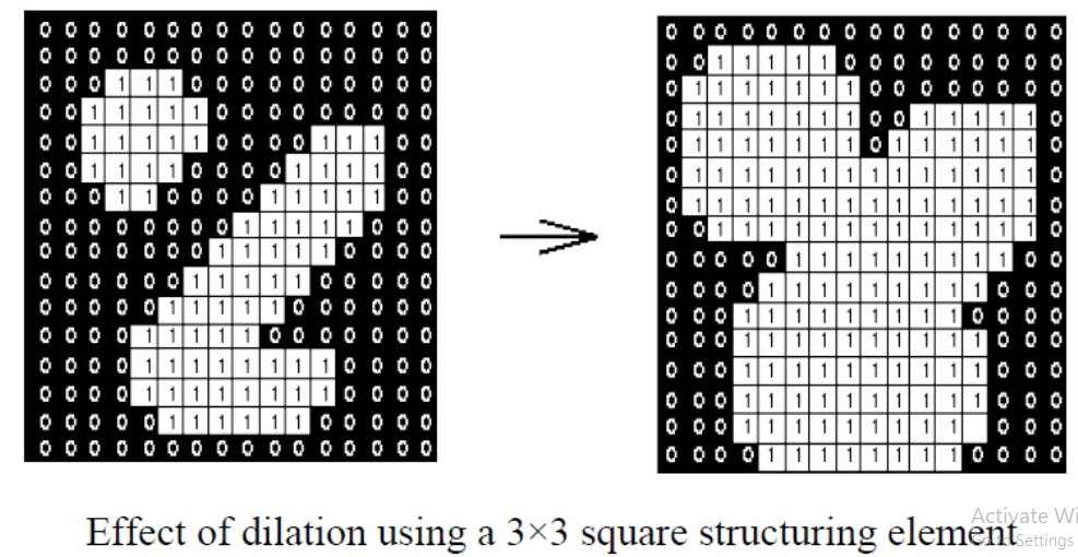
The basic idea is that the value of the output pixel is the maximum value of all the pixels in the input pixel's neighborhood. If any of the pixels in the kernel is 1, the pixel in the original image (under the kernel center) will be dilated (set to 1).

It's useful for joining broken parts of an object, filling small holes, and enhancing the boundaries of the foreground object.

In [27]:

dilated_image = cv2.dilate(image, kernel, iterations=1)
display_image_in_notebook(dilated_image)

dilated_image = cv2.dilate(image, kernel, iterations=1) display_image_in_notebook(dilated_image)

Erosion followed by dilation can help in removing noise it is often a good practice. This combination is known as "opening" 😎

In [29]:

opened_image = cv2.morphologyEx(image, cv2.MORPH_OPEN, kernel)
display_image_in_notebook(opened_image)

opened_image = cv2.morphologyEx(image, cv2.MORPH_OPEN, kernel) display_image_in_notebook(opened_image)

Erosion and dilation are powerful tools in morphological image processing. They provide a means to modify the geometric structure of objects in an image, enabling a wide range of applications from noise reduction to feature extraction. Understanding these operations is pivotal for anyone diving deep into image analysis and computer vision.

For a more in-depth understanding and exploration of advanced techniques, it's recommended to refer to OpenCV's official documentation and other image processing literature.