Introduction to OpenCV
What is Image Processing and Computer Vision ?

Image Processing
Image processing is a method to perform some operations on an image, in order to get an enhanced image or to extract some useful information from it. It's a type of signal processing in which the input is an image and the output is either an image or characteristics/features associated with that image. Image processing operations include smoothing, sharpening, contrasting, stretching, and edge detection, among others. These operations can be used to enhance the visibility of features, remove noise, prepare an image for further analysis, or achieve a variety of other effects.
Computer Vision
Computer vision is a field of artificial intelligence that enables computers and systems to derive meaningful information from digital images, videos, and other visual inputs, and based on those inputs, it can understand and automate tasks that the human visual system can do. While image processing and computer vision are distinct fields, they often overlap significantly, as both involve working with digital images.
Computer vision tasks include methods for acquiring, processing, analyzing, and understanding digital images and extraction of high-dimensional data from the real world in order to produce numerical or symbolic information.
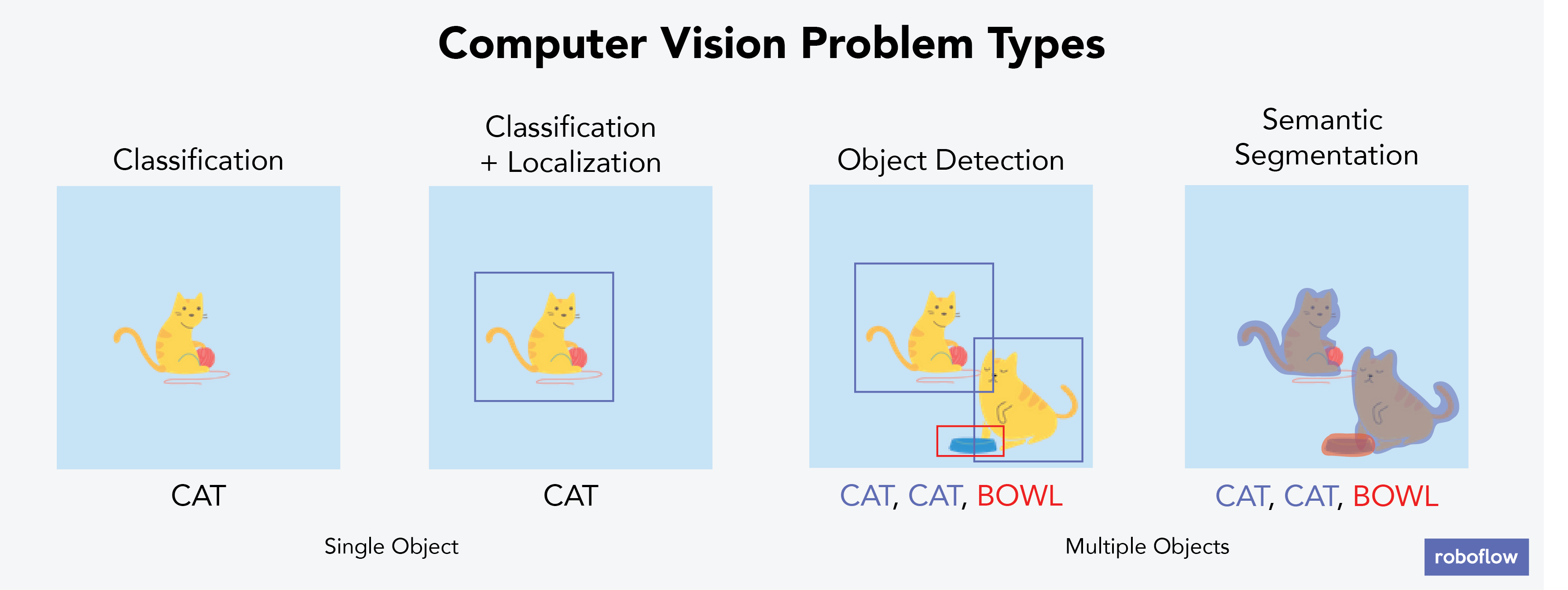
While us Humans can see and understand the world in 3D naturally, it is more difficult for computers 🤖 Indeed they need to break it into multiple small tasks like, image segmentation, classification, localization... By the way, researchers in computer vision have been developing mathematical techniques to recover the three-dimensional shape and ap- pearance of objects/scene from images.

But first thing first let's do some image processing in order to understand better how computers works with images and discover the OpenCV tool 😎
Machine Learning
Computer vision algorithms have seen a rapid progress in recent years. In particular, combining computer vision with machine learning contributes to the development of flexible and robust computer vision algorithms and, thus, improving the performance of practical vision systems.
For instance, Facebook has combined computer vision, machine learning, and their large corpus of photos, to achieve a robust and highly accurate facial recognition system. That is how Facebook can suggest who to tag in your photo. Same thing for Apple with the facial recognition for unlock your latest iPhone 🤓
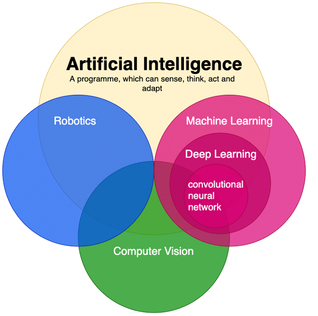
It is important to understand the similarities and the differences between theses fields like you can see in this figure bellow :

We will focus more on the Machine/Deep learning and CNNs in the end of this courses do not worry 🔥
Why OpenCV
OpenCV (Open Source Computer Vision) is a library of programming functions mainly aimed at real-time computer vision. This library is highly efficient and designed around real-time applications, and is widely used worldwide.
Installing OpenCV in Python
The easiest way to install OpenCV is via pip. If you have pip installed in your system, run the following command:
pip install opencv-python
If you want to install contrib modules along with OpenCV, use:
pip install opencv-contrib-python
How is an image encoded and read by computers
Gray VS Colors images
At the most basic level, a digital image is a two-dimensional grid of pixels. Each pixel represents the smallest piece of the image that we can control. The term pixel is derived from "picture element."
Each pixel in a grayscale image has a value representing the shade of gray. In an 8-bit image, this value ranges from 0 (black) to 255 (white). Thus, an 8-bit grayscale image can have 256 different possible shades of gray.
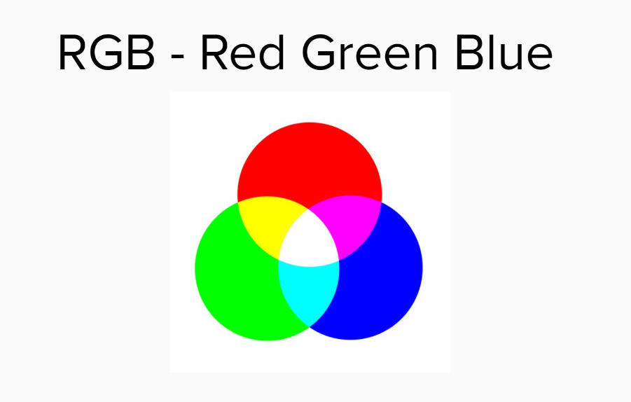
Color images are typically represented as a combination of red, green, and blue (the RGB color model). Each pixel in a color image is actually composed of three values (one for each of red, green, and blue), each of which can range from 0 to 255. Thus, an RGB image can represent more than 16 million unique colors. We will see this when we will print our images dimensions.

We will get back later on RGB don't worry 🤓
import numpy as np
import cv2

# Load an image
img = cv2.imread('./data/frame_1.png', 1)

# Print type of the image
print(type(img))  # Output: <class 'numpy.ndarray'>

# Print shape of the image
print(img.shape)  # Output for a color image: (height, width, channels)
<class 'numpy.ndarray'>
(1280, 720, 3)
As you can see, the image is represented as a numpy ndarray if it is not ringing a bell take a look at the numpy course 🤓.
The shape of the array is (height, width, channels), where the number of channels is 3 for a color image (blue, green, red).
Each pixel in the image is represented by a triplet of numbers, representing the blue, green, and red intensities, respectively.
Basic operations with images
Let's first learn the basics : load an image, print it (with matplotlib) and play with it 😎
Let's begin with writing a little helper function display_image_in_notebook to print the images here :
import cv2
import matplotlib.pyplot as plt

def display_image_in_notebook(img):
    # Convert the image from BGR to RGB
    img_rgb = cv2.cvtColor(img, cv2.COLOR_BGR2RGB)
    # Display the image using matplotlib
    plt.imshow(img_rgb)
    #plt.axis('off')
    plt.show()
# Load an image
img = cv2.imread('./data/frame_1.png', 1)

# Display the image in Jupyter notebook
display_image_in_notebook(img)
Accessing and modifying pixel values
You can access a pixel value by its row and column coordinates. For a BGR image, it returns an array of Blue, Green, Red values.
img
array([[[ 82,  87,  80],
        [ 85,  90,  83],
        [ 83,  88,  81],
        ...,
        [  7,   4,   0],
        [  6,   2,   0],
        [  7,   3,   0]],

       [[ 82,  87,  80],
        [ 85,  90,  83],
        [ 85,  90,  83],
        ...,
        [  7,   4,   0],
        [  8,   4,   0],
        [  9,   5,   1]],

       [[ 82,  87,  80],
        [ 82,  87,  80],
        [ 86,  91,  84],
        ...,
        [ 10,   7,   1],
        [ 13,   9,   5],
        [ 12,   8,   4]],

       ...,

       [[220, 220, 220],
        [221, 221, 221],
        [223, 223, 223],
        ...,
        [ 58,  54,  18],
        [ 53,  54,   9],
        [ 52,  53,   8]],

       [[167, 167, 167],
        [166, 166, 166],
        [165, 165, 165],
        ...,
        [ 46,  41,   0],
        [ 47,  48,   0],
        [ 47,  48,   0]],

       [[147, 147, 147],
        [142, 142, 142],
        [131, 131, 131],
        ...,
        [ 54,  49,   7],
        [ 53,  54,   2],
        [ 51,  52,   0]]], dtype=uint8)
# accessing pixel values
px = img[100, 100]
print(px)
[38 42 37]
#display only a specific part of the image using slicing
display_image_in_notebook(img[100:900,:430])
Resize and cropping images
#print the shape of the image
img.shape
(1280, 720, 3)
#random size you can change it if you want
new_width = 720
new_height = 540
resized_img = cv2.resize(img, (new_width, new_height))
display_image_in_notebook(resized_img)
#cropping
y_start = 0
y_end = 960
x_start = 100
x_end = -1
cropped_img = img[y_start:y_end, x_start:x_end]
display_image_in_notebook(cropped_img)
Encoding colors
Color spaces in image processing serve a crucial role: they provide a standardized method for specifying and representing colors. By defining colors in a consistent manner, these spaces ensure that colors are interpreted and displayed uniformly across different devices and platforms.
Different color models or spaces find their applications in various domains, from hardware design to software applications, including animation creation, digital art, photography, and video processing. Let's delve into some of the most common color models and understand their unique characteristics and applications.
RGB (Red, Green, Blue)
- Description: RGB is an additive color model where colors are produced by combining red, green, and blue light sources in various intensities.
- Application: Widely used in electronic displays like TVs, computer monitors, and cameras. It's the standard for digital imaging and graphic design.
CMYK (Cyan, Magenta, Yellow, Key/Black)
- Description: CMYK is a subtractive color model used in color printing. Unlike RGB, where colors are produced by adding light, in CMYK colors emerge by subtracting light (or, more precisely, by absorbing certain wavelengths of light and reflecting others).
- Application: Predominantly used in color printing processes, including magazines, brochures, and other printed materials.
HSV (Hue, Saturation, Value)
- Description: HSV represents colors in terms of their shades (hue), the intensity of the shade (saturation), and the brightness of the light (value). It's more intuitive for humans to understand and manipulate than RGB.
- Application: Often used in graphics software, especially in color pickers, because of its intuitive nature. It's also beneficial in computer vision tasks where color segmentation is required.
YIQ
- Description: YIQ splits an image's color information into a luminance component (Y) and two chrominance components (I and Q). It was designed to be compatible with black-and-white television while offering improved color representation.
- Application: Historically used in NTSC (National Television System Committee) broadcasts in North America. While not as commonly used today, understanding YIQ can be essential for working with older video technologies or archival footage.
Color filtering, or color detection, is one of the most fundamental operations in computer vision. It refers to identifying objects in an image based on color. In real-world images, color values can vary due to different lighting conditions, shadows, and even noise added by the camera during image capture and processing.
To accommodate these variations, we can perform color detection in an other color space like HSV (Hue, Saturation, Value) color space instead of the traditional RGB (Red, Green, Blue) color space.
In this course we will focus only on RGB and HSV encoding techniques in OpenCV.
RGB Encoding
As you may notice, the RGB color model is the predominant choice in digital image processing, including within OpenCV. This model breaks down a color image into three distinct channels, each dedicated to one of the primary colors: Red, Green, and Blue. Every other color emerges from varying combinations of these three foundational hues. In this system, a value of 0 signifies black, and as this value escalates, so does the intensity of the color.

An RGB image can be represented as a 3D matrix (or a 3D array) in Python, where the dimensions represent the height, width, and color channels of the image, respectively.
Here's a simple example using Python's NumPy library to represent a 3x3 RGB image:
# Define a 3x3 RGB image
# Each element [R, G, B] is a list of three integers (0-255)
image = np.array([
    [[255, 0, 0], [0, 255, 0], [0, 0, 255]],  # Red, Green, Blue
    [[255, 255, 0], [0, 255, 255], [255, 0, 255]],  # Yellow, Cyan, Magenta
    [[128, 128, 128], [64, 64, 64], [192, 192, 192]]  # Gray shades
])

print(image)
[[[255   0   0]
  [  0 255   0]
  [  0   0 255]]

 [[255 255   0]
  [  0 255 255]
  [255   0 255]]

 [[128 128 128]
  [ 64  64  64]
  [192 192 192]]]
# We can also see this image like this
plt.imshow(image)
<matplotlib.image.AxesImage at 0x12204ecc0>
HSV Encoding
The HSV color space separates image intensity (i.e., luminance or brightness) from the color information. The advantage of this separation is that it allows us to focus on the color spectrum while ignoring luminance. This capability is especially valuable when dealing with real-world images where lighting conditions can vary dramatically.
In the HSV color space, Hue represents the color, Saturation represents the amount to which that respective color is mixed with white, and Value represents the amount to which the color is mixed with black (or the brightness of the color).

🚧 In OpenCV, Hue values range from 0 to 180 (in contrast to 0 to 360 in many other applications as you can see on the picture above), and Saturation and Value are within the range 0 to 255. 🚧
OpenCV provides the function cv2.inRange(src, lowerb, upperb) to perform color detection. It takes three arguments:
src: the source array, in our case, the target HSV image.lowerb: the lower boundary array, an array of 3 values representing the lower range of HSV values.upperb: the upper boundary array, an array of 3 values representing the upper range of HSV values
This function generates a binary mask where pixels within the specified HSV range are set to 255 (white), and pixels outside this range are set to 0 (black)
You can then use this mask to filter the original image, displaying only the desired color using the function cv2.bitwise_and(src1, src2, mask). Now, let's put everything together with some Python code. We will detect the color red in an image.
# Load the image
image = cv2.imread('./data/frame_1.png', 1)

# Convert the image from BGR to HSV color space
image_hsv = cv2.cvtColor(image, cv2.COLOR_BGR2HSV)

# Define the lower and upper boundaries for the color red
# Lower boundary RED color range values; Hue (0 - 10)
lower_red1 = np.array([0, 100, 20])
upper_red1 = np.array([10, 255, 255])

# Upper boundary RED color range values; Hue (160 - 180)
lower_red2 = np.array([160,100,20])
upper_red2 = np.array([179,255,255])

# Create masks for the lower and upper red color ranges
mask_lower_red = cv2.inRange(image_hsv, lower_red1, upper_red1)
mask_upper_red = cv2.inRange(image_hsv, lower_red2, upper_red2)

# Combine the masks
mask_red = mask_lower_red + mask_upper_red

# Apply the mask to the image using bitwise_and operation
image_red = cv2.bitwise_and(image, image, mask=mask_red)

# Display the original and filtered images
display_image_in_notebook(image)
display_image_in_notebook(image_red)
You can easily apply this technique for various tasks such as object detection, image segmentation, and even tracking objects in real-time video. We will see later this part and try to track the red marker on the top of the stem in a video 🤔
By the way, if you pay attention you can notice our little red marker on the second image in a black backgroud 🥳
Keep in mind that the accuracy of color detection can be affected by various factors, including lighting conditions, shadows, and camera noise. You might need to adjust the HSV ranges for different environments to achieve the best results.
greenBGR = np.uint8([[[0,255,0 ]]])
hsv_green = cv2.cvtColor(greenBGR,cv2.COLOR_BGR2HSV)
display_image_in_notebook(greenBGR)
display_image_in_notebook(hsv_green)
As you can see the green colour is very different from an encoding to an other for us humans 🤖