Sorting Algorithms
Sorting Algorithms help rearrange a specific array or list based on a set rule that compares its elements. This rule determines how the elements should be organized within that structure.
For instance, consider a list of characters arranged based on their ASCII values in ascending order. This means characters with lower ASCII values come before those with higher values.
There is a wide range of sorting algorithms, each with its own advantages and disadvantages. Some are more efficient than others, and some are more suitable for certain types of data. Let's take a look at some of the most common sorting algorithms. In order to not be overwhelmed in a interview, we will only cover the most common ones.

Bubble Sort
The BubbleSort compares each successive pair of elements in an unordered list and inverts the elements if they are not in order. As you can see on the GIF bellow, the largest element will "bubble" to the end of the list after each iteration. This is why it is called BubbleSort.

Let's take a look ar a simple example of BubbleSort on the list [6,5,3,1,8,7,2,4] (pairs that were compared in each step are encapsulated in '**'):
{6,5,3,1,8,7,2,4}
{**5,6**,3,1,8,7,2,4} -- 5 < 6 -> swap
{5,**3,6**,1,8,7,2,4} -- 3 < 6 -> swap
{5,3,**1,6**,8,7,2,4} -- 1 < 6 -> swap
{5,3,1,**6,8**,7,2,4} -- 8 > 6 -> no swap
{5,3,1,6,**7,8**,2,4} -- 7 < 8 -> swap
{5,3,1,6,7,**2,8**,4} -- 2 < 8 -> swap
{5,3,1,6,7,2,**4,8**} -- 4 < 8 -> swap
After one iteration through the list, we have [5,3,1,6,7,2,4,8]. Note that the greatest unsorted value in the array (8 in this case) will always reach its final position. Thus, to be sure the list is sorted we must iterate $n-1$ times for lists of length n.
You can get more details about the pseudo code and implementation here.
%time
input_list = [10,1,2,11,4,7,8,3,43]

for i in range(len(input_list)):
    for j in range(i):
        if int(input_list[j]) > int(input_list[j+1]):
            input_list[j],input_list[j+1] = input_list[j+1],input_list[j]

input_list
CPU times: user 1e+03 ns, sys: 0 ns, total: 1e+03 ns
Wall time: 3.1 µs
[1, 2, 4, 7, 8, 3, 10, 11, 43]
QuickSort
The QuickSort algorithm that picks an element ("the pivot") and reorders the array forming two partitions such that all elements less than the pivot come before it and all elements greater come after. The algorithm is then applied recursively to the partitions until the list is sorted.
You can see this video of people dancing and sorting themselves to understand how the algorithm works, and to have a laugh also 😂
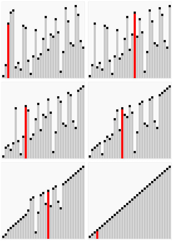
More seriously, you can see the same gif like the bubble sort but with quick sort below:

As you can see on the gif the quick sort is much more efficient than the bubble sort 😂
The quicksort algorithm is based on the divide and conquer principle even if it is a sorting algorithm. The pivot can be chosen in different ways, but the most common is to choose the last element of the array.
Then, we will iterate through the array and compare each element to the pivot. If the element is smaller than the pivot, we will swap it with the first element of the array that is greater than the pivot. This way, we will have all the elements smaller than the pivot on the left of the pivot, and all the elements greater than the pivot on the right of the pivot. Then, we will repeat the same process on the left and right subarrays until the array is sorted.
Let's dive into a python implementation of the quick sort algorithm:
%time
input_list = [10,1,2,11,4,7,8,3,43]

def quick_sort(array):
    if len(array) < 2:
        return array
    else:
        pivot = array[-1]
        smaller, equal, larger = [], [], []
        for i, num in enumerate(array):
            if num < pivot:
                smaller.append(num)
            elif num == pivot:
                equal.append(num)
            else:
                larger.append(num)
            # to see how the list is splitted in each iteration
            #print(f'split {i} | pivot : {pivot}, smaller: {smaller}, equal: {equal}, larger: {larger}')
        return quick_sort(smaller) + equal + quick_sort(larger)

quick_sort(input_list)
CPU times: user 1 µs, sys: 0 ns, total: 1 µs
Wall time: 2.15 µs
[1, 2, 3, 4, 7, 8, 10, 11, 43]
As you can see even for a tiny list of 9 elements, the quick sort is much more efficient than the bubble sort 🔥
Merge Sort
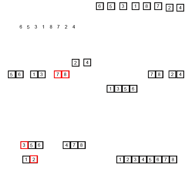
The Merge Sort algorithm is based on the divide and conquer principle also. It divides the array into two halves, sorts them recursively, and then merges the two sorted halves. It is very similar to the QuickSort algorithm, but instead of sorting the array in place, it creates two subarrays and merges them at the end.

def merge_sort(arr):
    """
    This function implements the Merge Sort algorithm.

    Parameters:
    - arr: List of elements to be sorted.

    Returns:
    - List of elements sorted in ascending order.
    """

    if len(arr) <= 1:
        return arr

    # Split the list in half
    mid = len(arr) // 2
    left_half = arr[:mid]
    right_half = arr[mid:]

    # Recursively sort both halves
    left_half = merge_sort(left_half)
    right_half = merge_sort(right_half)

    # Merge the sorted halves with right and left index pointers
    merged = []
    left_index, right_index = 0, 0

    while left_index < len(left_half) and right_index < len(right_half):
        if left_half[left_index] < right_half[right_index]:
            merged.append(left_half[left_index])
            left_index += 1
        else:
            merged.append(right_half[right_index])
            right_index += 1

    # Append any remaining elements from both halves (one of them will be empty)
    while left_index < len(left_half):
        merged.append(left_half[left_index])
        left_index += 1

    while right_index < len(right_half):
        merged.append(right_half[right_index])
        right_index += 1

    return merged

%time
input_list = [10,1,2,11,4,7,8,3,43]
merge_sort(input_list)
CPU times: user 1e+03 ns, sys: 0 ns, total: 1e+03 ns
Wall time: 1.91 µs
[1, 2, 3, 4, 7, 8, 10, 11, 43]
As you can see the merge sort is efficient also, pretty much the same time as the quick sort. The time complexity of the merge sort is $O(nlog(n))$.