Searching algorithms¶

Searching algorithms are a category of algorithms that deal with the problem of locating a specific item or set of items from a collection. This collection can be in any data structure like arrays, lists, or even trees and graphs for specific problems.

The searching problem is one of the fundamental computer science problems that is used extensively in computer science and has a wide variety of applications. For example, the searching problem is used in the Google search engine to search for web pages containing a specific keyword. More information on Wikipedia here.

In this chapter, we will discuss the following topics :

• Linear Search
• Binary Search
• Jump Search
• Interpolation Search
• Sublist Search (Search a linked list in another list)
• Graph Search

First thing first, let's take a look at the linear search algorithm.

Linear Search¶

Linear search is a very simple search algorithm. In this type of search, a sequential search is made over all items one by one. Every item is checked and if a match is found then that particular item is returned, otherwise the search continues till the end of the data collection. In term of complexity, linear search is a very basic search algorithm with the worst case performance of $O(n)$, so it's not very efficient for large data collection, like you can see from this meme 😅

The most intuitive form of searching is a linear search as you may know. Let's write a function linear_search(arr: list, x: int) -> int that searches for x in arr and returns the index of x if found, otherwise -1.

Input: arr = [2, 4, 6, 8, 10], x = 6
Output: 2

In [4]:

def linear_search(arr, x):
    for i in range(len(arr)):
        if arr[i] == x:
            return i
    return -1

%time
linear_search([2, 4, 6, 8, 10],6)

def linear_search(arr, x): for i in range(len(arr)): if arr[i] == x: return i return -1 %time linear_search([2, 4, 6, 8, 10],6)

CPU times: user 3 µs, sys: 0 ns, total: 3 µs
Wall time: 6.91 µs

Out[4]:

2

Binary search¶

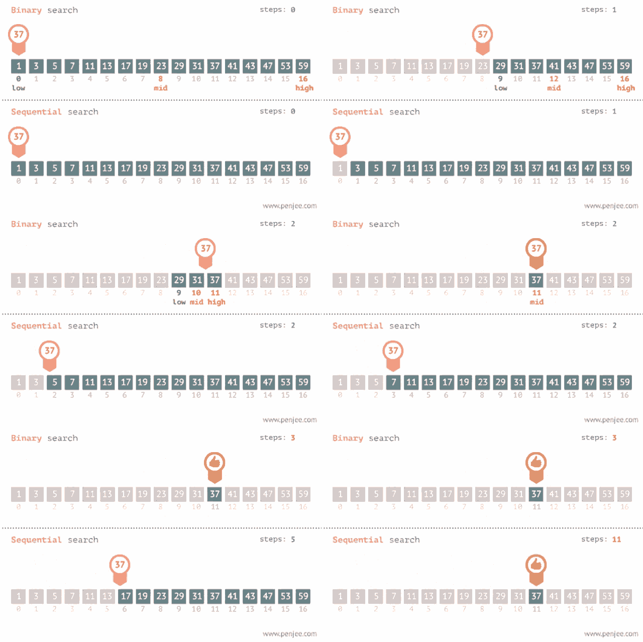
Binary search is an efficient algorithm for finding an item from a sorted list of items. It works by repeatedly dividing the portion of the list that could contain the item until you've narrowed down the possible locations to just one. More details on Wikipedia here.

Because a picture worth a thousand words, let's take a look at this animation to understand how binary search works.

Let's try to write a function binary_search(arr: list, x: int) -> int that do the same task as before, searches for x in a sorted arr and returns the index of x if found, otherwise -1.

Input: arr = [1, 3, 5, 7, 9], x = 7
Output: 3

In [5]:

def binary_search(arr, x):
    low = 0
    high = len(arr) - 1
    mid = 0
    while low <= high:
        mid = (high + low) // 2
        if arr[mid] < x:
            low = mid + 1
        elif arr[mid] > x:
            high = mid - 1
        else:
            return mid
    return -1

%time
binary_search([2, 4, 6, 8, 10],6)

def binary_search(arr, x): low = 0 high = len(arr) - 1 mid = 0 while low <= high: mid = (high + low) // 2 if arr[mid] < x: low = mid + 1 elif arr[mid] > x: high = mid - 1 else: return mid return -1 %time binary_search([2, 4, 6, 8, 10],6)

CPU times: user 1 µs, sys: 0 ns, total: 1 µs
Wall time: 2.15 µs

Out[5]:

2

Jump search¶

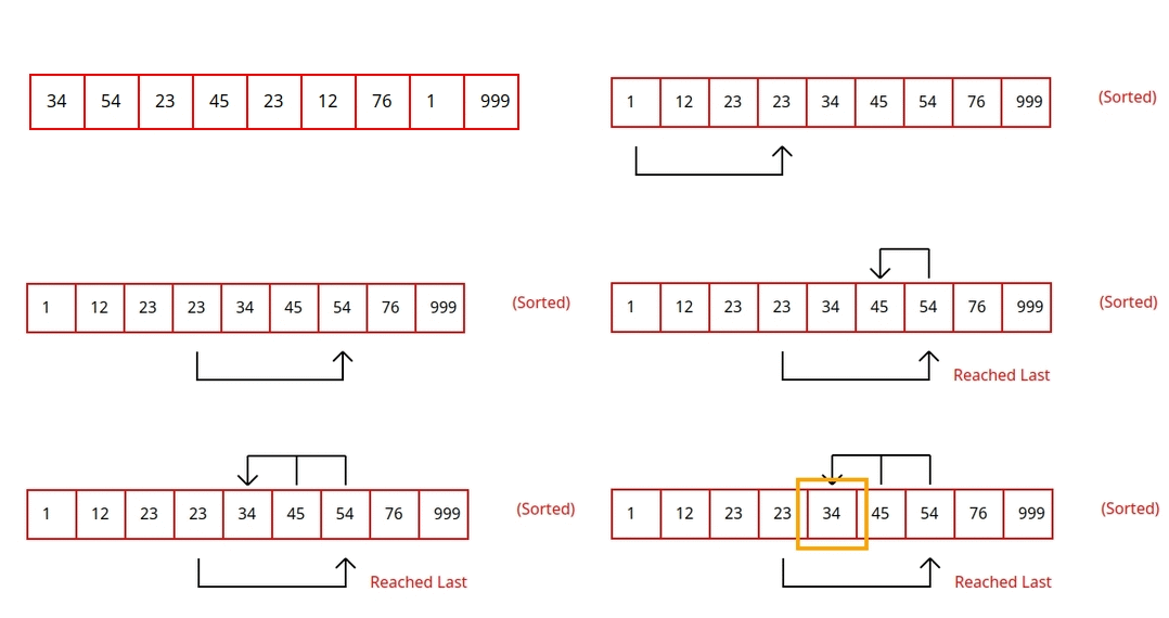
Jump search is a searching algorithm for sorted arrays. The basic idea is to check fewer elements by jumping ahead fixed steps like you can see in this animation below.

Write a function jump_search(arr: list, x: int) -> int that searches for x in a sorted arr and returns the index of x if found, otherwise -1.

In [10]:

import math

def jump_search(arr, x):
    length = len(arr)
    #  we defined the jump as the square root of the length of the array for the first jump
    jump = int(math.sqrt(length))
    prev, curr = 0, 0

    while curr < length and arr[curr] <= x:
        prev, curr = curr, min(curr + jump, length)

    for i in range(prev, curr):
        if arr[i] == x:
            return i
    return -1


%time
jump_search([2, 4, 6, 8, 10],6)

import math def jump_search(arr, x): length = len(arr) # we defined the jump as the square root of the length of the array for the first jump jump = int(math.sqrt(length)) prev, curr = 0, 0 while curr < length and arr[curr] <= x: prev, curr = curr, min(curr + jump, length) for i in range(prev, curr): if arr[i] == x: return i return -1 %time jump_search([2, 4, 6, 8, 10],6)

CPU times: user 1e+03 ns, sys: 0 ns, total: 1e+03 ns
Wall time: 2.86 µs

Out[10]:

2

Interpolation search¶

Interpolation search is an improved variant of binary search. This search algorithm works on the probing position of the required value. For this algorithm to work properly, the data collection should be in a sorted form and equally distributed. You can read more about it on Wikipedia here before continuing.

Let's write a function interpolation_search(arr: list, x: int) -> int for the same task as before.

In [11]:

def interpolation_search(arr, x):
    low, high = 0, len(arr) - 1

    while low <= high and x >= arr[low] and x <= arr[high]:
        if low == high:
            if arr[low] == x:
                return low
            return -1

        pos = low + int(((float(high - low) / (arr[high] - arr[low])) * (x - arr[low])))
        if arr[pos] == x:
            return pos
        if arr[pos] < x:
            low = pos + 1
        else:
            high = pos - 1
    return -1

%time
interpolation_search([2, 4, 6, 8, 10],6)

def interpolation_search(arr, x): low, high = 0, len(arr) - 1 while low <= high and x >= arr[low] and x <= arr[high]: if low == high: if arr[low] == x: return low return -1 pos = low + int(((float(high - low) / (arr[high] - arr[low])) * (x - arr[low]))) if arr[pos] == x: return pos if arr[pos] < x: low = pos + 1 else: high = pos - 1 return -1 %time interpolation_search([2, 4, 6, 8, 10],6)

CPU times: user 1e+03 ns, sys: 0 ns, total: 1e+03 ns
Wall time: 1.91 µs

Out[11]:

2

Sublist Search¶

Sublist Search is a searching algorithm that searches for a linked list in another list. It is also known as the single-link list search algorithm, you can read more about linked list on Wikipedia here.

First thing first we need to define a linked list as a python class and then we can write a function is_sublist(list1: ListNode, list2: ListNode) -> bool that checks if list1 is a sublist of list2.

Input:
list1 = 1 -> 2 -> 3
list2 = 3 -> 4 -> 1 -> 2 -> 3 -> 5
Output: True

In [13]:

class ListNode:
    def __init__(self, value=0, next=None):
        self.value = value
        # we define next as None by default
        self.next = None

def is_sublist(list1, list2):
    if not list1:
        return True
    if not list2:
        return False
    
    # we initialize two pointers to traverse the lists
    ptr1 = list1
    ptr2 = list2

    # we traverse the second list until we find the first element of the first list
    while ptr2:
        if ptr2.value == ptr1.value:
            temp_ptr1 = ptr1
            temp_ptr2 = ptr2
            while temp_ptr1 and temp_ptr2 and temp_ptr1.value == temp_ptr2.value:
                temp_ptr1 = temp_ptr1.next
                temp_ptr2 = temp_ptr2.next
            if not temp_ptr1:
                return True
        ptr2 = ptr2.next
    return False

# Helper function to create a linked list from a list of values
def create_linked_list(values):
    if not values:
        return None
    head = ListNode(values[0])
    current = head
    for value in values[1:]:
        current.next = ListNode(value)
        current = current.next
    return head

list1 = create_linked_list([1, 2, 3])
list2 = create_linked_list([3, 4, 1, 2, 3, 5])
is_sublist(list1, list2)

class ListNode: def __init__(self, value=0, next=None): self.value = value # we define next as None by default self.next = None def is_sublist(list1, list2): if not list1: return True if not list2: return False # we initialize two pointers to traverse the lists ptr1 = list1 ptr2 = list2 # we traverse the second list until we find the first element of the first list while ptr2: if ptr2.value == ptr1.value: temp_ptr1 = ptr1 temp_ptr2 = ptr2 while temp_ptr1 and temp_ptr2 and temp_ptr1.value == temp_ptr2.value: temp_ptr1 = temp_ptr1.next temp_ptr2 = temp_ptr2.next if not temp_ptr1: return True ptr2 = ptr2.next return False # Helper function to create a linked list from a list of values def create_linked_list(values): if not values: return None head = ListNode(values[0]) current = head for value in values[1:]: current.next = ListNode(value) current = current.next return head list1 = create_linked_list([1, 2, 3]) list2 = create_linked_list([3, 4, 1, 2, 3, 5]) is_sublist(list1, list2)

Out[13]:

True

Graph Search¶

Graph search algorithms are a category of algorithms that deal with the problem of searching a specific item or set of items from a graph or a tree data structure.

Graphs are a common data structure that consists of nodes and edges. Searching is a fundamental operation on them. If you don't know what is a graph, you can read more about it on Wikipedia here).

Let's take a look to the first simple search in Graph structure : Depth First Search (DFS) is a common algorithm to traverse or search through graphs 🤓

Depth First Search (DFS) and Breadth First Search (BFS)¶

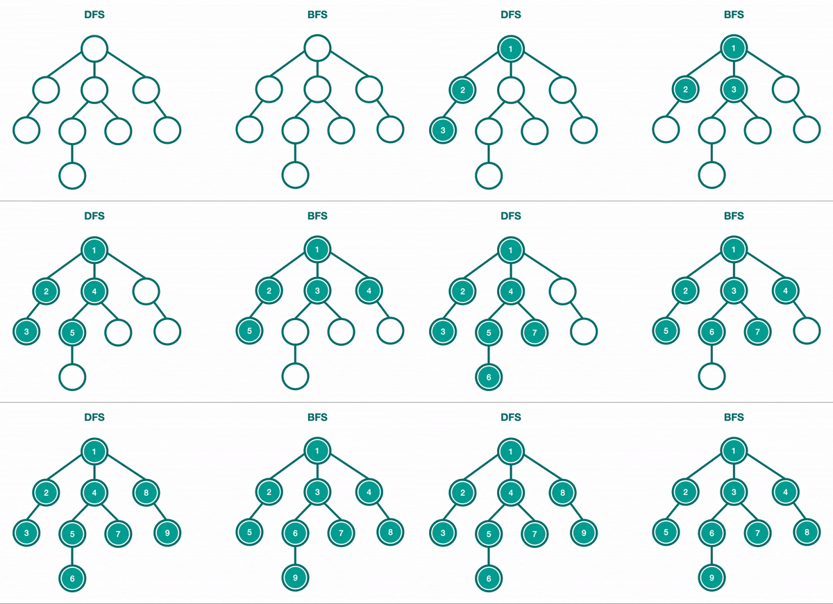
Depth First Search (DFS) and Breadth First Search (BFS) are common algorithms who starts at the root node (selecting some arbitrary node as the root node in the case of a graph) and explores as far as possible along each branch before backtracking. So the basic idea is to start from the root or any arbitrary node and mark the node and move to the adjacent unmarked node and continue this loop until there is no unmarked adjacent node. Then backtrack and check for other unmarked nodes and traverse them. Finally print the nodes in the path. The algorithm can works either recursively or iteratively on graphs and trees.

You can see on this animation below how DFS and BFS works on a tree structure :

Let's implements these two algorithms in python here :

In [31]:

def DFS(graph, start):
    visited = set()
    stack = [start]
    output = []

    while stack:
        vertex = stack.pop()
        if vertex not in visited:
            visited.add(vertex)
            output.append(vertex)
            stack.extend(reversed(graph[vertex]))
    return output

def BFS(graph, start):
    visited = set()
    queue = [start]
    output = []

    while queue:
        vertex = queue.pop(0)
        if vertex not in visited:
            visited.add(vertex)
            output.append(vertex)
            queue.extend(graph[vertex])
    return output

# We will define the graph as a dictionary with node as key and its neighbors as values
graph = {0: [1, 2], 1: [2], 2: [0, 3], 3: [3]}

def DFS(graph, start): visited = set() stack = [start] output = [] while stack: vertex = stack.pop() if vertex not in visited: visited.add(vertex) output.append(vertex) stack.extend(reversed(graph[vertex])) return output def BFS(graph, start): visited = set() queue = [start] output = [] while queue: vertex = queue.pop(0) if vertex not in visited: visited.add(vertex) output.append(vertex) queue.extend(graph[vertex]) return output # We will define the graph as a dictionary with node as key and its neighbors as values graph = {0: [1, 2], 1: [2], 2: [0, 3], 3: [3]}

In [16]:

# uncomment the following line to install networkx the library for graph algorithms and visualization
#! pip install networkx

# uncomment the following line to install networkx the library for graph algorithms and visualization #! pip install networkx

Requirement already satisfied: networkx in ./anaconda3/lib/python3.9/site-packages (2.8.4)

In [18]:

import networkx as nx
import matplotlib.pyplot as plt

def draw_graph(graph):
    G = nx.DiGraph(graph)  # Create a directed graph using networkx
    pos = nx.spring_layout(G)  # Define a layout for our graph
    
    # Draw nodes, edges, and labels
    nx.draw_networkx_nodes(G, pos)
    nx.draw_networkx_edges(G, pos)
    nx.draw_networkx_labels(G, pos)

    plt.title("Our Graph Visualization")
    plt.show()

graph = {0: [1, 2], 1: [2], 2: [0, 3], 3: [3]}
draw_graph(graph)

import networkx as nx import matplotlib.pyplot as plt def draw_graph(graph): G = nx.DiGraph(graph) # Create a directed graph using networkx pos = nx.spring_layout(G) # Define a layout for our graph # Draw nodes, edges, and labels nx.draw_networkx_nodes(G, pos) nx.draw_networkx_edges(G, pos) nx.draw_networkx_labels(G, pos) plt.title("Our Graph Visualization") plt.show() graph = {0: [1, 2], 1: [2], 2: [0, 3], 3: [3]} draw_graph(graph)

In [32]:

def test_graph_search():
    graph = {0: [1, 2], 1: [2], 2: [0, 3], 3: [3]}

    # Test DFS
    dfs_result = DFS(graph, 2)
    print("DFS Result:", dfs_result)
    assert dfs_result == [2, 0, 1, 3]

    # Test BFS
    bfs_result = BFS(graph, 2)
    print("BFS Result:", bfs_result)
    assert bfs_result == [2, 0, 3, 1]

    print("All tests passed!")

test_graph_search()

def test_graph_search(): graph = {0: [1, 2], 1: [2], 2: [0, 3], 3: [3]} # Test DFS dfs_result = DFS(graph, 2) print("DFS Result:", dfs_result) assert dfs_result == [2, 0, 1, 3] # Test BFS bfs_result = BFS(graph, 2) print("BFS Result:", bfs_result) assert bfs_result == [2, 0, 3, 1] print("All tests passed!") test_graph_search()

DFS Result: [2, 0, 1, 3]
BFS Result: [2, 0, 3, 1]
All tests passed!

Other searching algorithms¶

Keep in mind that searching algorithms are a very large category of algorithms and there are many other algorithms that we didn't cover in this chapter. You can find more information about them on Geeksforgeeks here.

For each data structure, there are many searching algorithms that are more efficient depending on your use case. For example, for a sorted array, we can use binary search, interpolation search, etc. For a tree, we can use binary search tree and for a graph, we can use A* search or Dijkstra's but we will cover these algorithms in the graph section.